SQL + Python + Spark for Data Science

··

42 min read

Table of Content:
Prerequisites:
A). Pyspark Connection - skip this section:
B). Create dataframe by reading files and datatype conversion - skip this section:
- B1). Create Student dataframe and define datatypes in pyspark:
- B2). Create University dataframe and define datatypes in pyspark:
- B3). Create Company dataframe and define datatypes in pyspark:
- B4). Create Year_Month_Day dataframe and define datatypes in pyspark:
C). Create TempView(Table), Data overview and size(count)- skip this section:
- C1). Student_Table Schema, Row count, Data Overview:
- C2). Student_Table Schema, Row count, Data Overview:
- C3). Company_Table Schema, Row count, Data Overview:
- C4). Year_Month_Day_Table Schema, Row count, Data Overview:
D). Select statement ( * , AS, LIMIT, COUNT(), DISTINCT ):
- D1). Select only few columns + LIMIT:
- D2). Select all the columns + LIMIT:
- D3). Alias names for columns :
- D4). Counting number of records:
- D5). Select some random text:
- D6). Distinct in select statement:
E). Where clause(BETWEEN, LIKE, IN, AND, OR):
- E1). WHERE clause:
- E2). WHERE clause + BETWEEN:
- E3). WHERE clause + LIKE:
- E4). WHERE clause + IN:
- E5). WHERE clause + AND:
- E6). WHERE clause + OR:
F). Order By:
- F1). ORDER BY + ASC:
- F2). ORDER BY + DESC:
G). Upper(), Lower(), Length() functions:
H). Concatenation(||) + BooleanExpression + TRIM() functions:
- H1). Concatenation (||):
- H2). Boolean Expression:
- H3). TRIM() function:
I). SUBSTRING() + REPLACE() + POSITION() functions:
- I1). SUBSTRING() function:
- I2). REPLACE() function:
- I3). POSITION() function:
J). Aggregation functions:
- J1). COUNT() function:
- J2). MAX() function:
- J3). MIN() function:
- J4). SUM(), AVG() functions:
K). GROUP BY + HAVING clauses:
- K1). GROUP BY Example-1:
- K2). GROUP BY Example-2:
- K3). GROUP BY + Having:
L). Sub Queries:
- L1). Subquery Example-1:
M). Correlated sub queries:
- M1). Correlated sub query Example-1:
N). Case statement:
- N1). Case Statement Example-1:
O). Joins (INNER, LEFT, RIGHT, FULL, CROSS):
- O1). Joins concept overview with Example-1:
- O2). INNER JOIN:
- O3). LEFT JOIN:
- O4). RIGHT JOIN:
- O5). FULL OUTER JOIN:
- O6). CROSS JOIN:
P). Union, Union all, Except:
- P1). UNION:
- P2). UNION ALL:
- P3). EXCEPT:
Q). Window functions:
- Q1). ROW_NUMBER() Example-1 without Partition:
- Q2). ROW_NUMBER() Example-2 with Partition:
- Q3). RANK:
- Q4). DENSE_RANK():
- Q5). ROW_NUMBER, RANK, DENSE_RANK in single output:
- Q6). NTILE:
- Q7). LEAD:
- Q8). LAG:
- Q9). Running aggregation functions in window functions(COUNT(), SUM(), AVG(), MIN(), MAX()):
Conclusion:

Table of Content:

In this SQL tutorial, we will be learning below concepts. As I've used Jupyter-Notebooks for writing this blog I've used Pyspark for interactive outputs. so just to skip Pyspark stuff directly jump to Section-D for SQL concepts.
Note: I've used some dummy data so that we can cover all SQL concepts with all edge cases.

Prerequisites:
A). Pyspark Connection - skip this section:
B). Create dataframe by reading files and datatype conversion - skip this section:
C). Create TempView(Table), Data overview and size(count)- skip this section:
D). Select statement (*, AS, LIMIT, COUNT(), DISTINCT):
E). Where clause(BETWEEN, LIKE, IN, AND, OR):
F). Order By:
G). Upper(), Lower(), Length() functions:
H). Concatenation(||) + BooleanExpression + TRIM() functions:
I). SUBSTRING() + REPLACE() + POSITION() functions:
J). Aggregation functions:
K). GROUP BY + HAVING:
L). Sub Queries:
M). Correlated sub queries:
N). Case statement:
O). Joins (INNER, LEFT, RIGHT, FULL, CROSS):
P). Union, Union all, Except:
Q). Window functions:
Conclusion:

Prerequisites:

Basic understanding of rows, columns in table or excel sheet will be enough to understand the SQL concepts. To get more insight about the data we have, by using SQL (Structure Query Language) we can get quick detailed analysis.

Note: Here we are using Python+Spark+SQL to get the output.
Spark: Is In-Memory processing engine from Apache for Big data analysis.
Python: As a programming language(scripting language) we are using with Spark.
SQL: for querying data to get required outputs.

In every section just see the sql_query line to understand the concepts. Rest of the codes are written in Pyspark to print the output in Jupyter-notebooks. In general if we have any software for RDBMS, we no need to worry about the Pyspark codes. You can directly jump to D section to begin the SQL concepts.

A). Pyspark Connection - skip this section:

#Connection part for Pyspark and importing required packages.
import pandas as pd
import numpy as np

from pyspark.sql import SparkSession
from pyspark.sql.types import *
from pyspark.sql.functions import *
from pyspark.sql import *

spark = SparkSession.builder.appName("Pyspark_with_SQL").getOrCreate()
conf = spark.sparkContext._conf.setAll([('spark.driver.memory', '4g'), ('spark.executor.memory', '4g'), ('spark.executor.num','6'), ('spark.network.timeout', '1000000')])

Explanation: Spark is in-memory data processing analytics engine. Spark is mainly used in Bigdata platforms to process the large data in less running time. It is having parallel processing capacity due to this we can given required number of executors(just like threads in multi-threading concepts) to distribute the data parallelly and execute(process) the largge amount of data in less time.
Spark offers 4 languages to write the frameworks. These are Python, Java, R, Scala. In this blog we are using Python + Spark so called Pyspark. Above syntax is used to create spark session so that, we can able to query the SQL commands directly using Python and we are intimating how many executors(Threads in multi-threading) required in this session. For now we can skip this section and jump to section-D.

B). Create dataframe by reading files and datatype conversion - skip this section:

In this blog we are having 4 datasets(tables in SQL) mentioned below. Before creating a dataset(table), we are assigning the datatype for each column in each table. Here with the help of Pandas, Pyspark dataframes we are defining datatypes for each column. Lets work on each table.

Student table: contains all Student related information. Excel file link here.
University table: contains all University related information. Excel file link here.
Company table: contains all Company related information. Excel file link here.
Year_Month_Day table: contains sample data for Date type related information. Excel file link here.

B1). Create Student dataframe and define datatypes in pyspark:

student_dfpd = pd.read_excel(r'Table_Source\Student_Placement_Table.xlsx')

schema_student = StructType([\
                     StructField("ID",IntegerType(),False),\
                     StructField("Name",StringType(),False),\
                     StructField("Gender",StringType(),False),\
                     StructField("DOB",DateType(),False),\
                     StructField("Location",StringType(),True),\
                     StructField("University",StringType(),False),\
                     StructField("Salary",DoubleType(),False),\
                     StructField("Company",StringType(),False),\
                     StructField("Email",StringType(),False)])

student_dfps = spark.createDataFrame(student_dfpd, schema_student)

Explanation:

Line-1: Using pd.read_excel() method reading the excel file and creating pandas dataframe.
Line-2: Using StructType and StructField we are defining the schema for the dataset (datatype for each column names and whether it is nullable or not). Ex: For ID column we are informing that it is integer type and it cannot be null(means ID column shouldn't have missing data in it.)
Line-3: Using spark.createDataFrame() method with data, schema parameters we are creating Pyspark dataframe.

B2). Create University dataframe and define datatypes in pyspark:

university_dfpd = pd.read_excel(r'Table_Source\University_Table.xlsx')

schema_university = StructType([\
                     StructField("University",StringType(),False),\
                     StructField("MinSalary",StringType(),False),\
                     StructField("PlayGround",StringType(),False),\
                     StructField("Total_Students",IntegerType(),False)])

university_dfps = spark.createDataFrame(university_dfpd, schema_university)

Explanation:

Line-1: Using pd.read_excel() method reading the excel file and creating pandas dataframe.
Line-2: Using StructType and StructField we are defining the schema for the dataset (datatype for each column names and whether it is nullable or not). Ex: For Total_Students column we are informing that it is integer type and it cannot be null(means Total_Students column shouldn't have missing data in it.)
Line-3: Using spark.createDataFrame() method with data, schema parameters we are creating Pyspark dataframe.

B3). Create Company dataframe and define datatypes in pyspark:

company_dfpd = pd.read_excel(r'Table_Source\Company_Table.xlsx')

schema_company = StructType([\
                     StructField("Company",StringType(),False),\
                     StructField("Total_Employes",IntegerType(),False),\
                     StructField("Total_Products",IntegerType(),False),\
                     StructField("Hike_Per_Anum",IntegerType(),False),\
                     StructField("WHF_Office",StringType(),False)])

company_dfps = spark.createDataFrame(company_dfpd, schema_company)

Explanation:

Line-1: Using pd.read_excel() method reading the excel file and creating pandas dataframe.
Line-2: Using StructType and StructField we are defining the schema for the dataset (datatype for each column names and whether it is nullable or not). Ex: For Total_Employes column we are informing that it is integer type and it cannot be null(means Total_Employes column shouldn't have missing data in it.)
Line-3: Using spark.createDataFrame() method with data, schema parameters we are creating Pyspark dataframe.

B4). Create Year_Month_Day dataframe and define datatypes in pyspark:

year_month_day_dfpd = pd.read_excel(r'Table_Source\Year_Month_Day.xlsx')

schema_year_month_day = StructType([\
                     StructField("Year",IntegerType(),False),\
                     StructField("Month",StringType(),False),\
                     StructField("Day",IntegerType(),False),\
                     StructField("Salary",IntegerType(),False)])

year_month_day_dfps = spark.createDataFrame(year_month_day_dfpd, schema_year_month_day)

Explanation:

Line-1: Using pd.read_excel() method reading the excel file and creating pandas dataframe.
Line-2: Using StructType and StructField we are defining the schema for the dataset (datatype for each column names and whether it is nullable or not). Ex: For Year column we are informing that it is integer type and it cannot be null(means Year column shouldn't have missing data in it.)
Line-3: Using spark.createDataFrame() method with data, schema parameters we are creating Pyspark dataframe.

C). Create TempView(Table), Data overview and size(count)- skip this section:

In this section we are creatingPyspark TempView(just like Table in SQL) and cross checking the table schema, sample data and record count. Below code snippet is for creating temporary views in pyspark with the help of pyspark dataframe we created in previous sections.

student_dfps.createOrReplaceTempView("Student_Table")
university_dfps.createOrReplaceTempView("University_Table")
company_dfps.createOrReplaceTempView("Company_Table")
year_month_day_dfps.createOrReplaceTempView("Year_Month_Day_Table")

Explanation: Here we are creating TempViews for all above 4 pyspark dataframes so that in coming sections we can directly work on SQL queries. In each line left side we have pyspark dataframe name. In Pyspark we have createOrReplaceTempView() method to create Table like structure so that we can work on SQL queries to get the required information.
EX: Lets take first line, where student_dfps is the pyspark dataframe, Student_Table is the pyspark temporary view where we can apply all SQL stuff on top of it.
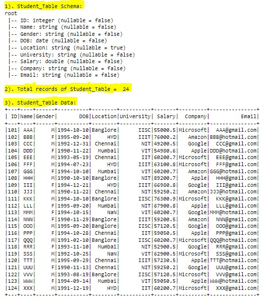
Now lets check the each table schema, record count and sample data.

C1). Student_Table Schema, Row count, Data Overview:

#print("Student_Table Schema:")
student_dfps.printSchema()

#print total count of records 
print("Total records of Student_Table = ",student_dfps.count(),"\n\nStudent_Table Data:")

#List all the records in table
sql_query = "SELECT * FROM Student_Table"
spark.sql(sql_query).show(30)

Explanation:

Command-1: Using printSchema() method we can able to view the schema for all columns in the dataframe with nullable check.
Command-2: Using count() method we can check the row count for pyspark dataframe.
Command-3: sql_query is a python string variable it contains actual SQL query to perform.
Command-4: Using spark.sql() method we can send the actual SQL command to execute and provide the output. show() method is used to limit the records(rows) to be printed. If we skip to provide the value, bydefault it will print first 20 records only. It is like LIMIT clause in SQL. If dataframe record count is lessthan given parameter or default(20 count) then it will only print the available records in table.
Output:

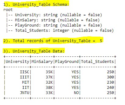
C2). Student_Table Schema, Row count, Data Overview:

#print("1). University_Table Schema:")
university_dfps.printSchema()

#print total count of records 
print("2). Total records of University_Table = ",university_dfps.count(),"\n\n3). University_Table Data:")

#List all the records in table
sql_query = "SELECT * FROM University_Table"
spark.sql(sql_query).show(30)

Explanation:

Command-1: Using printSchema() method we can able to view the schema for all columns in the dataframe with nullable check.
Command-2: Using count() method we can check the row count for pyspark dataframe.
Command-3: sql_query is a python string variable it contains actual SQL query to perform.
Command-4: Using spark.sql() method we can send the actual SQL command to execute and provide the output. show() method is used to limit the records(rows) to be printed. If we skip to provide the value, bydefault it will print first 20 records only. It is like LIMIT clause in SQL. If dataframe record count is lessthan given parameter or default(20 count) then it will only print the available records in table.
Output:

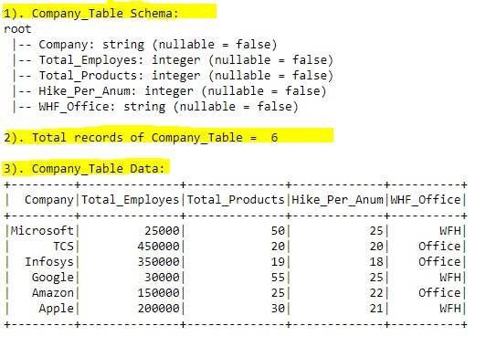
C3). Company_Table Schema, Row count, Data Overview:

#print("1). Company_Table Schema:")
company_dfps.printSchema()

#print total count of records 
print("2). Total records of Company_Table = ",company_dfps.count(),"\n\n3). Company_Table Data:")

#List all the records in table
sql_query = "SELECT * FROM Company_Table"
spark.sql(sql_query).show(30)

Explanation:

Command-1: Using printSchema() method we can able to view the schema for all columns in the dataframe with nullable check.
Command-2: Using count() method we can check the row count for pyspark dataframe.
Command-3: sql_query is a python string variable it contains actual SQL query to perform.
Command-4: Using spark.sql() method we can send the actual SQL command to execute and provide the output. show() method is used to limit the records(rows) to be printed. If we skip to provide the value, bydefault it will print first 20 records only. It is like LIMIT clause in SQL. If dataframe record count is lessthan given parameter or default(20 count) then it will only print the available records in table.
Output:

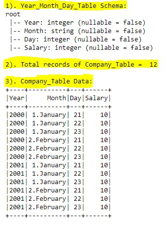
C4). Year_Month_Day_Table Schema, Row count, Data Overview:

#print("1). Year_Month_Day_Table Schema:")
year_month_day_dfps.printSchema()

#print total count of records 
print("2). Total records of Company_Table = ",year_month_day_dfps.count(),"\n\n3). Company_Table Data:")

#List all the records in table
sql_query = "SELECT * FROM Year_Month_Day_Table"
spark.sql(sql_query).show(30)

Explanation:

Command-1: Using printSchema() method we can able to view the schema for all columns in the dataframe with nullable check.
Command-2: Using count() method we can check the row count for pyspark dataframe.
Command-3: sql_query is a python string variable it contains actual SQL query to perform.
Command-4: Using spark.sql() method we can send the actual SQL command to execute and provide the output. show() method is used to limit the records(rows) to be printed. If we skip to provide the value, bydefault it will print first 20 records only. It is like LIMIT clause in SQL. If dataframe record count is lessthan given parameter or default(20 count) then it will only print the available records in table.
Output:

D). Select statement ( `*` , AS, LIMIT, COUNT(), DISTINCT ):

Select statement is used to select(choose or print) the few columns or all columns from the table. Lets explore all edge cases with select statement.

*: used to select all the columns from the table.
AS: used to alias the column name in output console.
LIMIT: used to limit the records in output console for mentioned columns.
count(*): used to print the valid record count from the table.
DISTINCT: used to fetch unique values from the table for mentioned column(s).

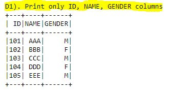
D1). Select only few columns + LIMIT:

#print("D1). Print only ID, NAME, GENDER columns")

sql_query="""
SELECT ID, NAME, GENDER 
FROM Student_Table 
LIMIT 5
"""
spark.sql(sql_query).show()

Explanation: Here we have mentioned specific column names we want to print in output rather all the columns from the table with LIMIT clause so that number of records will be filters to given number(20). This will help in selecting required columns and provide the output to business in real time.
Output:

D2). Select all the columns + LIMIT:

#print("D2). Print all columns from table only 5 rows.")

sql_query="""
SELECT * 
FROM Student_Table 
LIMIT 5
"""

spark.sql(sql_query).show()

Explanation: By using * in the select statement we can fetch all the columns available in table to output. By using LIMIT we are restricting number of records in output for given number. Here it is 5 rows with all the columns.
Output:

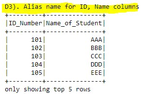
D3). Alias names for columns :

#print("D3). Alias name for ID, Name columns")

sql_query="""
SELECT ID as ID_Number, Name as Name_of_Student 
FROM Student_Table
"""

spark.sql(sql_query).show(5)

Explanation: Sometimes table might contains very short column names which cannot be understand or sometimes column name might be very lengthy which can be understand in short name in this case we can use Alias names for the columns using AS keyword. Here ID column is printed as ID_Number column , Name column printed as Name_of_Student column. This Alias concept will give some temporary names for the columns unless we use this concept in inner queries so that original column names will be remain same for the table.
Output:

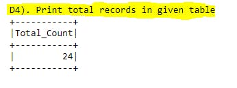
D4). Counting number of records:

#print("D4). Print total records in given table")

sql_query="""
SELECT count(*)as Total_Count 
FROM Student_Table
"""

spark.sql(sql_query).show()

Explanation: Here we are using count(*) as a column name called Total_Count. This will give us the number of valid (not - null)records available in the table. If we use count(1) in the select query then it will valid(not-null) records in the first column of the table. This will be very handy to check how many missing values present in given column from the table. If we missing giving number and mentioned as * it means that it will check all the columns missing data for all rows(if and only if in single row all columns data having null then only it will skip that record while counting) and print the valid records from the table.
Output:

D5). Select some random text:

#print("D5). Print some sample text using select statement")

sql_query="""
SELECT 'Hello I am SQL' as Column_Name 
"""

spark.sql(sql_query).show()

Explanation: Selecting some random text will be very useful in real time when we apply UNION, UNION ALL statements and one of the table having more columns than other in that case we case this kind of temporary data and alias to the matching column from other table so that UNION statements will not impact and gives the output. Here Hello I am SQL is the data in the column called Column_Name.

Output:

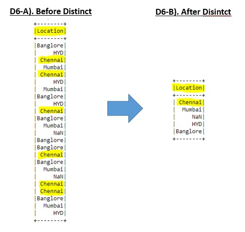
D6). Distinct in select statement:

#print("D6-A). Without Distinct statement, it will list all records in that column(s)")

sql_query="""
SELECT Location 
FROM Student_Table
"""

spark.sql(sql_query).show(30)


#print("D6-B). With Distinct statement, it will list only distinct records in that column(s)")

sql_query="""
SELECT DISTINCT Location 
FROM Student_Table
"""

spark.sql(sql_query).show(30)

Explanation: If we want to check for unique values in a single column or unique values with combination of multiple columns we can use DISTINCT keyword. Ex: In Location column we have value Chennai has been repeated 6 times. After applying DISTINCT we could see only once in the output.
Output:

E). Where clause(BETWEEN, LIKE, IN, AND, OR):

With select statement we can restrict the number of columns to be printed.
With where clause we can restrict the number of records(rows) to be printed.

Based on some condition(s), if we want to filter the data we can use WHERE clause. This is totally different than LIMIT clause because with LIMIT we cannot filter the data based on conditions it simply restrict the row count for given numbers. WHERE clause is frequently used in real time analysis because business table will be containing all sort of data and based on filter conditions we can get the required data out of it. Lets explore different ways to use WHERE clause.

BETWEEN: To filter the data with given range.
LIKE: To filter the data for given data pattern.
IN: To filter the data for given list of values.
AND: To filter the data for both conditions becomes true.
OR: To filter the data for any one conditions becomes true.

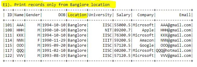
E1). WHERE clause:

#print("E1). Print records only from Banglore location")

sql_query="""
SELECT * 
FROM Student_Table 
WHERE Location = 'Banglore' 
"""

spark.sql(sql_query).show()

Explanation: If the scenario is filter the data for Banglore location we can use the above syntax to get required output.
Output:

E2). WHERE clause + BETWEEN:

#print("E2). Print records only ID range from 105 to 109 Inclusive")

sql_query="""
SELECT * 
FROM Student_Table 
WHERE ID BETWEEN 105 AND 109
"""

spark.sql(sql_query).show()

Explanation: Here by using BETWEEN command with WHERE clause we could able to print the ID's from 105 to 109 inclusively. Even if few ID's are present in table then those condition matching records will be printed.
Output:

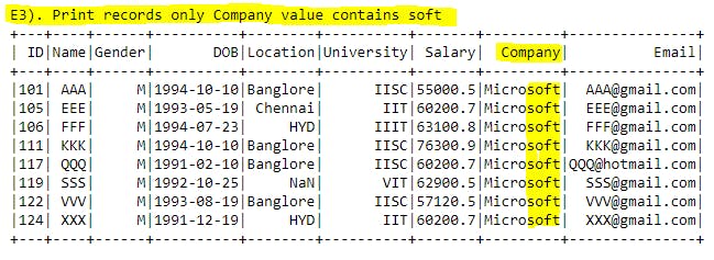
E3). WHERE clause + LIKE:

#print("E3). Print records only Company value contains soft")

sql_query="""
SELECT * 
FROM Student_Table 
WHERE COMPANY LIKE "%soft%" 
"""

spark.sql(sql_query).show()

Explanation: By using LIKE command with WHERE clause we can able to filter the data with given patterns for any columns data. Here we could able to print the company names which have soft substring within COMPANY column value.
Output:

E4). WHERE clause + IN:

#print("E4). Print records only Name in given list(AAA, GGG, KKK)")

sql_query="""
SELECT * 
FROM Student_Table 
WHERE NAME IN ('AAA', 'GGG', 'KKK') 
"""

spark.sql(sql_query).show()

Explanation: With BETWEEN command we will give the range for the column to be filtered. But in IN command we will be giving the list of values to be checked for WHERE condition.
Output:

E5). WHERE clause + AND:

#print("E5). Print records from Banglore location and Microsoft company")

sql_query="""
SELECT * 
FROM Student_Table 
WHERE (
              LOCATION ='Banglore' AND 
              COMPANY ='Microsoft'
              ) 
"""

spark.sql(sql_query).show()

Explanation: With WHERE clause if we use AND command then given all conditions should be matched for the output. Both the conditions should be TRUE. Ex: Here the conditions are LOCATION ='Banglore' AND COMPANY ='Microsoft' and in the all the records with there two conditions will be printed.
Output:

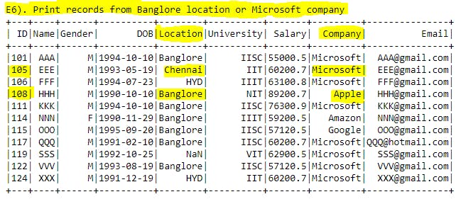
E6). WHERE clause + OR:

#print("E6). Print records from Banglore location or Microsoft company")

sql_query="""
SELECT * 
FROM Student_Table 
WHERE (
              LOCATION ='Banglore' OR 
              COMPANY ='Microsoft'
              ) 
"""

spark.sql(sql_query).show()

Explanation: Difference between AND, OR is in AND command if and only if given 2 conditions should be matched then only that record will be printed in the output. But in OR command either of the conditions matches then matching record will be printed in the output. Ex: Here Even if Location= 'Chennai' also printed in the output because in that record Company='Microsoft' so here one condition is matching and so that record will be printed in the output.
Output:

F). Order By:

In real time data analysis ordering the data based on one column or combination of columns has been frequently used for business solutions. By default ORDER BY clause will sort the data in ascending order or explicitly we can use the keyword called ASC.

ASC : will sort the data in ascending order for given column(s).
DESC: will sort the data in descending order for given column(s).

F1). ORDER BY + ASC:

#print("F1). Sort by Salary Accending order top 5 records")

sql_query="""
SELECT * 
FROM Student_Table 
ORDER BY Salary ASC
LIMIT 5
"""

spark.sql(sql_query).show()

Explanation: By default with ORDER BY clause follows ascending order. Just for our understanding we can use ASC keyword after the column name(s). In Ascending order integers, floats will start from 0 to n and string values will be sorted from A to Z. If any special characters there in the column values then ASCII values will come to the picture. Ex: In below example we are sorting the salaries in ascending order.
Output:

F2). ORDER BY + DESC:

#print("F2). Sort by Name Descending order top 5 records")

sql_query="""
SELECT * 
FROM Student_Table 
ORDER BY Name DESC 
LIMIT 5
"""

spark.sql(sql_query).show()

Explanation: By using DESC key word we can sort the data in descending order. In this case integers, floats will start from n to 0 and string values will be sorted from Z to A. Ex: In below we are sorting Names in descending order.
Output:

G). Upper(), Lower(), Length() functions:

For string valued columns we can apply these functions. Lets see the below description for given function.

UPPER(): string data will be converted to upper case.
LOWER(): string data will be converted to lower case.
LENGTH(): for string data it will give the character length in numbers.

Lets explore these functions with real time data.

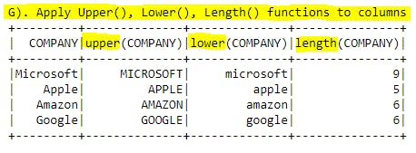
#print("G). Apply Upper(), Lower(), Length() functions to columns")

sql_query="""
SELECT DISTINCT COMPANY, 
UPPER(COMPANY), 
LOWER(COMPANY), 
LENGTH(COMPANY) 
FROM Student_Table
"""

spark.sql(sql_query).show()

Explanation: In this example we used COMPANY column's data applied DISTINCT keyword to restrict the duplicates.

In first column data will come as is.
In second column data will be converted into upper case.
In third column data will be converted into lower case.
In forth column, we get the number of characters in each record data. Ex: Apple is having 5 characters. Here empty spaces will also be considered for counting.

Output:

H). Concatenation(||) + BooleanExpression + TRIM() functions:

Lets check on some useful functions which are frequently used in real time data analysis.

Concatenation (||): To club multiple columns or strings into single column.
BooleanExpression: After applying boolean expression on some column to get True or False values.
TRIM(): To eliminate the spaces between string columns.

H1). Concatenation (||):

#print("H1). Concatenation using || symbol and club multiple columns into single column.")

sql_query="""
SELECT Name, University, 'I am ' || Name || ' from ' || University as Self_Intro 
FROM Student_Table 
LIMIT 10
"""

spark.sql(sql_query).show()

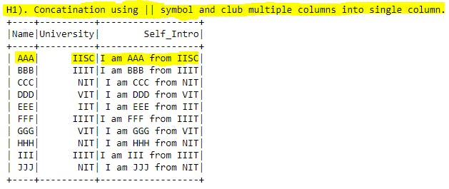
Explanation: By using concatenation symbol || we can club Name, Universitycolumns and few strings into Self_Intro column. Here 'I am ' || Name || ' from ' || University is mapped to single column.
Output:

H2). Boolean Expression:

#print("H2). Boolean Expression with some condition")

sql_query="""
SELECT ID, NAME, SALARY, (Salary > 60000) As IsSalaryGraterThan60K 
FROM Student_Table 
LIMIT 10
"""

spark.sql(sql_query).show()

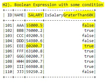
Explanation: By using conditional operators called =, !=, >, >=, <, <= we can apply conditions and create a new column to get the boolean values based on given condition. Here in below example we comparing the Salary column if it is more than 60,000 or not. If salary grater than 60,000 we will get true else false into new alias column we created called IsSalaryGraterThan60K.
Output:

H3). TRIM() function:

#print("H3). Trim() function used to remove extra spaces in column's data")

sql_query="""
SELECT 
'   Google    ' AS ExtraSpaces, LENGTH('   Google    ') AS Len_ExtraSpaces,
TRIM('   Google    ') AS TrimApplied, LENGTH(TRIM('   Google    ')) AS Len_TrimApplied,
RTRIM('   Google    ') AS RTrimApplied, LENGTH(RTRIM('   Google    ')) AS Len_RTrimApplied,
LTRIM('   Google    ') AS LTrimApplied, LENGTH(LTRIM('   Google    ')) AS Len_LTrimApplied
"""

spark.sql(sql_query).show()

Explanation: For our understanding I've added extra spaces before and after to Google word.

By using TRIM() function we can able to remove the extra spaces before and after to the word.
By using RTRIM() function we can able to remove extra spaces right side(after) the word.
By using LTRIM() function we can able to remove extra spaces left side(before) the word.

In below output we can easily relate the each section with function and its length function.

Output:

I). SUBSTRING() + REPLACE() + POSITION() functions:

These functions can be applied on String datatype columns. Lets explore each of these functions.

SUBSTRING() : To extract the given range substring from column.
REPLACE() : To replace the column existing data with given new data.
POSITION() : To give the exact the position(index) of the given string in columns data.

I1). SUBSTRING() function:

#print("I1).Extract IIIT from IIIT Banglore")

sql_query="""
SELECT 'IIIT Banglore' AS FullColumn, 
SUBSTRING('IIIT Banglore',1,4) AS SubstringColumn 
"""

spark.sql(sql_query).show()

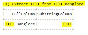
Explanation: By using SUBSTRING() function we can able to print substring value of any given columns data. Parameters are column name, starting position, number of characters has to be printed. If we observe SUBSTRING('IIIT Banglore',1,4) parameters are IIIT Banglore column name or column data, 1 is the starting position of string from left side, 4 is the number of characters has to be printed from starting position i.e. 1. So now totally 4 characters will be printed from left side starting postion i.e. IIIT.
Output:

I2). REPLACE() function:

#print("I2). Replace all IIIT to IIIT-B")

sql_query="""
SELECT ID, Name, University, 
REPLACE(UNIVERSITY, 'IIIT', 'IIIT-B')AS Replaced 
FROM Student_Table 
LIMIT 10
"""

spark.sql(sql_query).show()

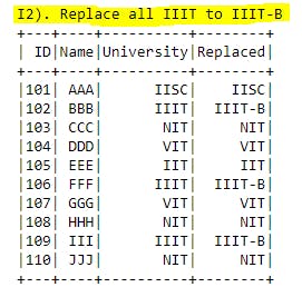
Explanation: By using REPLACE() function we can able to replace the data in given column with given data. Here we have used UNIVERSITY column name and IIIT is the existing data . Now we are replacing IIIT with IIIT-B and alias name for new column(alias names can be any thing as per our choice.) is Replaced.
Output:

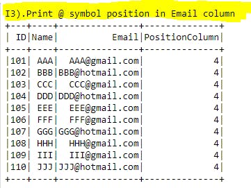
I3). POSITION() function:

#print("I3).Print @ symbol position in Email column")

sql_query="""
SELECT ID, Name, Email, POSITION('@' IN Email) AS PositionColumn 
FROM Student_Table 
LIMIT 10
"""

spark.sql(sql_query).show()

Explanation: We want to know the position of @ symbol in the POSITION column for each record. Here we have used POSITION('@' IN Email) as a syntax to get the positions of given string. @ is the string we are looking and Email is the column name we are searching for @ symbol. As an output we will get 4 for all the records because in all the records we could see @ in 4th index.
Output:

J). Aggregation functions:

For now lets focus on few aggregated functions which are not required to apply Group by, having clauses. In next section we will explore more on Aggregation functions with Group by, having clauses. Lets explore below functions one by one.
Note: These functions will be used in advanced analysis with window functions, Group by statements and many more that we are going to explore in the upcoming sections. Below few examples are very basic and outputs will be on top of entire table level but not for any specific column level aggregation. For column level aggregations we will group by statements in coming sections.

COUNT() : Will print the total record count for given scenario.
MAX(): Will print the maximum value in column for given scenario.
MIN() : Will print the minimum value in column for given scenario.
SUM() : Will print the summation value in column for given scenario.
AVG() : Will print the average value in column for given scenario.

J1). COUNT() function:

#print("J1).Print total number of records in the Student_Table table.")

sql_query="""
SELECT COUNT(*) 
FROM Student_Table
"""

spark.sql(sql_query).show()

Explanation: COUNT(*) function will print the total number of records available in the table.
Output:

J2). MAX() function:

#print("J2-a).Print Maximum value in Salary")
sql_query="""
SELECT MAX(Salary) AS MAX_Salary 
FROM Student_Table
"""
spark.sql(sql_query).show()


#print("J2-b).Check - Print Table Based on Salary Descending order ")
sql_query="""SELECT * FROM Student_Table ORDER BY Salary DESC LIMIT 5"""
spark.sql(sql_query).show()

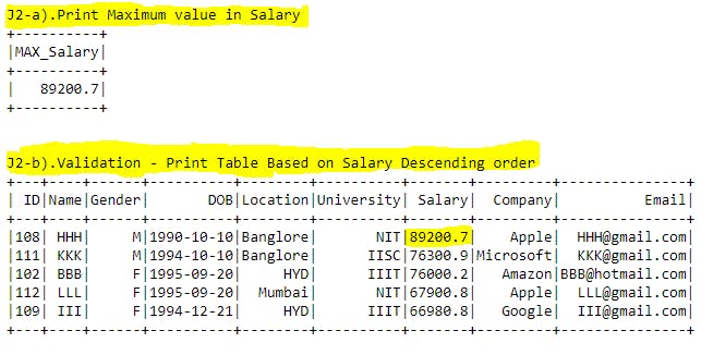
Explanation: In J2-a section we have applied the MAX() function on Salary column. In the output we could see the maximum salary from the table.
For validation purpose in J2-b section we are sorting the Salary column in descending order so that maximum salary record will come first. This kind of validation required in analytics field for all the concepts based on scenario we need to check with other approach to test the results are coming proper or not.
Output:

J3). MIN() function:

#print("J3-a).Print Minimum value in Salary")
sql_query="""
SELECT MIN(Salary) AS MIN_Salary 
FROM Student_Table
"""
spark.sql(sql_query).show()


#print("J3-b).Validation - Print Table Based on Salary Ascending order ")
sql_query="""SELECT * FROM Student_Table ORDER BY Salary LIMIT 5"""
spark.sql(sql_query).show()

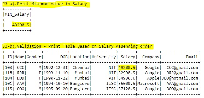
Explanation: In J3-a section we have applied the MIN() function on Salary column. In the output we could see the minimum salary from the table.
For validation purpose in J3-b section we are sorting the Salary column in ascending order so that minimum salary record will come first.
Output:

J4). SUM(), AVG() functions:

#print("J4-a).SUM(), AVG() functions")
sql_query="""
SELECT SUM(Salary) AS SumSalary, 
AVG(Salary) AS AverageSalary 
FROM Student_Table
"""
spark.sql(sql_query).show()


#print("J4-b).Validation for Average value based on sum value. (SUM/Total records)")
sql_query="""SELECT 1482743.7000000002/24 as validation"""
spark.sql(sql_query).show()

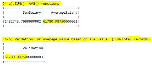
Explanation: By using SUM() function we can able to add all salaries from the table. By using AVG() function we can get the average value of salaries. For validation purpose we have checked the formula(Average = Sum/Total records) and both outputs are matching for Average value.
Output:

K). GROUP BY + HAVING clauses:

Till now we have used aggregations on table level. If we want to use 1 or more column level aggregations we will be using GROUP BY, HAVING clauses. Lets explore few examples on this topic. More option these GROUP BY, HAVING clauses can be used all together.

GROUP BY : To apply aggregations on column(s) level.
HAVING : To filter the outputs based on specific aggregated conditions.

K1). GROUP BY Example-1:

#print("K1).Print number of Students working in each company ")

sql_query="""
SELECT Company, count(*) TotalStudents_PerCompany 
FROM Student_Table 
GROUP BY Company
"""

spark.sql(sql_query).show()

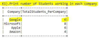
Explanation: We know that count(*) can be used to get the total records from table. But when we use count(*) with GROUP BY clause it will group the outputs into clusters of given group by column data distinct values and give the output accordingly.
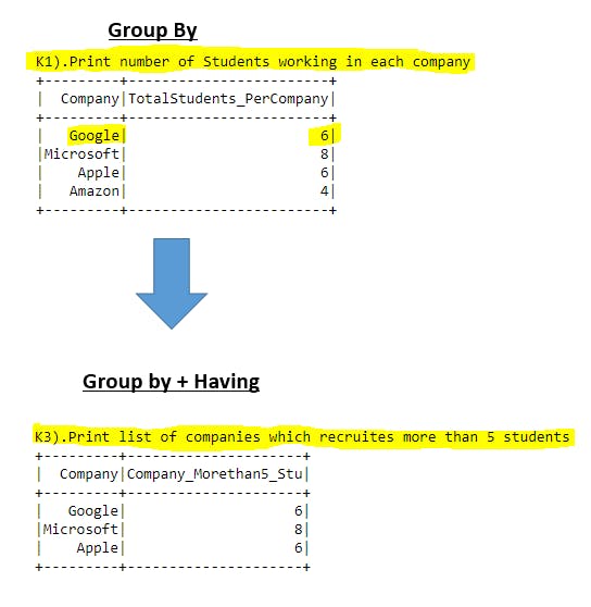
Ex: In this example we have used GROUP BY Company code so that outputs will be grouped into company distinct values and because of count(*) TotalStudents_PerCompany aggregated total students counts will be printed to each company. For example in Google company 6 students got placed.
Output:

K2). GROUP BY Example-2:

#print("K2).Print Total salary of Students based on company. Note:Round function used")

sql_query="""
SELECT Company, ROUND(SUM(Salary)) TotalSalary_PerCompany 
FROM Student_Table 
GROUP BY Company
"""

spark.sql(sql_query).show()

Explanation: This is similar example for above one. Here we want to know total salary offered by each company for all the students. Here we have applied SUM() function on Salary and we are grouping the output on Company column. So that in the output we will get total salary offered by each company.
Output:

K3). GROUP BY + Having:

#print("K3).Print list of companies which recruites more than 5 students")

sql_query="""
SELECT Company, COUNT(*) AS Company_Morethan5_Stu 
FROM Student_Table 
GROUP BY Company 
HAVING Company_Morethan5_Stu>5
"""

spark.sql(sql_query).show()

Explanation: If we see the K1 example, we have totally 4 companies w.r.t count of students got selected. Now by using Having clause we are filtering the aggregated results based on some condition. In the output we could see that those companies which hired morethan 5 students and Amazon company hired only 4 students and it is not there in the output.
Note: We cannot use filter the aggregated results with WHERE clause that is the reason we are using HAVING clause. We can use WHERE clause before GROUP BY to filter the data.
Output:

L). Sub Queries:

Subqueries can be used inside of the other SQL queries. We mainly see subqueries in SELECT or WHERE clauses of SQL queries. We mainly use subqueries to restrict the output of outer queries based on some condition.
Subquires and Joins are serve the same purpose of combining data from multiple tables but joins will be used to combine tables based on matching column from both the tables where as subqueries will restrict the records based on single value or list of values.
Subqueries will be enclosed with parenthesis ().

L1). Subquery Example-1:

#print("L1).Print Student details with uniersity having PlayGround.")
sql_query="""
SELECT * 
FROM Student_Table 
WHERE University IN(
                    SELECT University 
                    FROM University_Table 
                    WHERE PlayGround = 'YES'
                    )
"""
spark.sql(sql_query).show()


#print("L2).Cross verify which Universities have Playground.")
sql_query="""
SELECT University 
FROM University_Table 
WHERE PlayGround = 'YES' 
"""
spark.sql(sql_query).show()

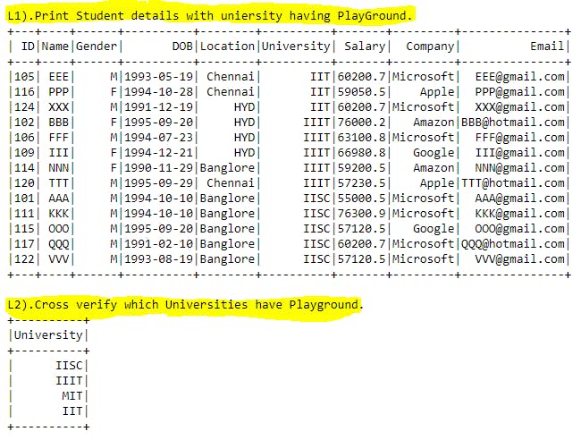
Explanation: Lets say we want to print all the students details where university should have PlayGround. By using where clause we can simply do this but Student_Table table doesn't have PlayGround details. In this scenario we are filtering the records of Student_Table by using subquery () in where clause. We have created subquery which only returns University names having PlayGround. Now outer query results restricted to subquery output values.
If we use subqueries in where clause we are simply passing 1 or more values to filter the data just like we did in basic where clause examples.

Output:

M). Correlated sub queries:

Correlated subqueries are similar to subqueries but in Correlated subqueries will be executed row by row i.e. each subquery will be executed once for each row of the outer query. This will take more time to provide the output. But in normal subqueries output of subquery will be generated first and send the values to outer query. Here subquery will not be executed morethan once.

M1). Correlated sub query Example-1:

#print("M1).Print Student details where university is in University table.")
sql_query="""
SELECT ID, Name, Email, Location, University
FROM Student_Table outer_query
WHERE EXISTS (
                    SELECT University 
                    FROM University_Table inner_query
                    WHERE inner_query.University = outer_query.University 
)                    
"""
spark.sql(sql_query).show()


#print("M2).Cross verify which Universities are in University_Table")
sql_query="""
SELECT University 
FROM University_Table
"""
spark.sql(sql_query).show()

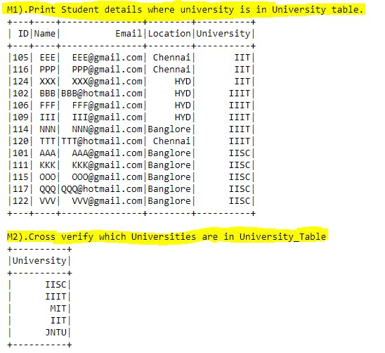
Explanation: Here in subquery we have used outer query matching filter to get the university details from University_Table. Due to this for each row of outerquery, the innerquery will be evaluated to check the given condition. This concept will take more time than normal subqueries. Insted of using this concept we need to check if there is any other alternative for this and use that concept.

Output:

N). Case statement:

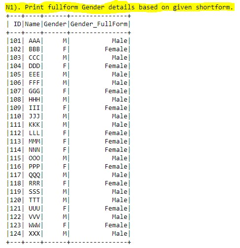
By using CASE statements we can able to create a new column with multiple if/else conditions by returning a value to the given conditions. It is similar to if, elif, else statements in any programming language. In SQL we apply these conditional flows by checking each row and assigning proper value in new column. Lets see an example to understand the concept.

N1). Case Statement Example-1:

#print("N1). Print fullform Gender details based on given shortform.")
sql_query="""
SELECT ID, Name, Gender,
CASE
    WHEN Gender = 'M' THEN 'Male'
    WHEN Gender = 'F' THEN 'Female'
    ELSE 'Other'
END Gender_FullForm  
FROM Student_Table
"""

spark.sql(sql_query).show()

Explanation: By using CASE statement we are creating Gender_FullForm column based on Gender existing column. Here we have used WHEN THEN as multiple if statements and ELSE as not matching values in WHEN THENstatements and END finishing followed by new column name we want to create. This concept will be very useful in real time data analysis to create new columns based on existing data conditions.
Output:

O). Joins (INNER, LEFT, RIGHT, FULL, CROSS):

When we want club columns from multiple tables based on matching criteria we will use Joins in SQL.
In most of time as a Data Analyst we spent time on connecting to multiple tables and bring all required columns in single table. Here JOINS will help us doing the same.
Joins concept used for clubbing multiple tables horizontally(combining columns) and UNION concepts used to club multiple tables vertically(combining rows).

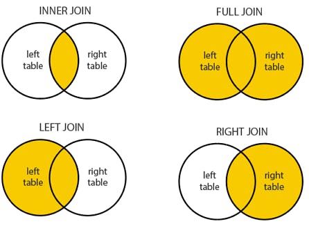
INNER JOIN : Returns records based on matching values in both tables.
LEFT JOIN : Returns all records from left table + matching records from right table.
RIGHT JOIN : Returns all records from right table + matching records from left table.
FULL JOIN : Returns all records from left table + right table.
CROSS JOIN : Returns Cartesian product of rows from both tables.

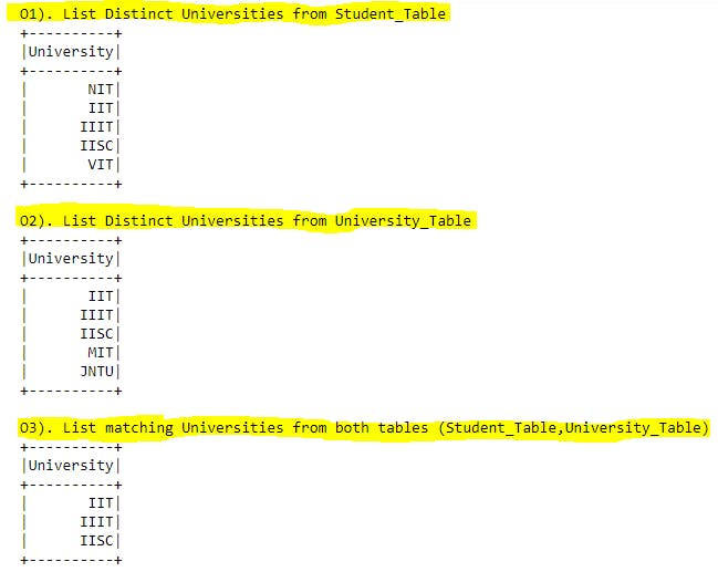
O1). Joins concept overview with Example-1:

#print("O1). List Distinct Universities from Student_Table")
sql_query="""
SELECT DISTINCT University 
FROM Student_Table
"""
spark.sql(sql_query).show()

#print("O2). List Distinct Universities from University_Table")
sql_query="""
SELECT DISTINCT University 
FROM University_Table
"""
spark.sql(sql_query).show()

#print("O3). List matching Universities from both tables (Student_Table,University_Table)")
sql_query="""
SELECT DISTINCT A.University 
FROM Student_Table A 
INNER JOIN University_Table B
ON A.University = B.University
"""
spark.sql(sql_query).show()

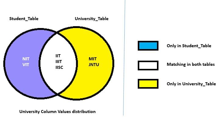
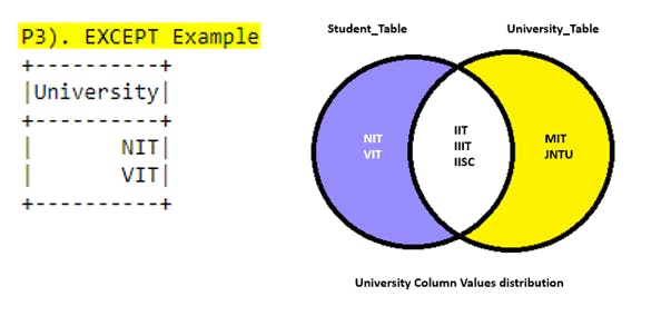
Explanation: In this Joins section, we will be using Student_Table , University_Table to apply joins concepts for University column. Before that if we observe below colorful diagram we will easily understand the JOINS easily. In both tables IIT, IIIT, IISC universities are matching. NIT, VIT only available in Student_Table(here we have matching universities aswell). MIT, JNTU only available in University_Table (here we have matching universities aswell).
Lets explore different types of JOINS with examples.

Output:

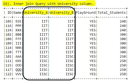
O2). INNER JOIN:

#print("O2). Inner join Query with University column.")
sql_query="""
SELECT A.ID, A.Name, A.University AS University_A, B.University AS University_B, B.PlayGround, B.Total_Students 
FROM Student_Table A 
INNER JOIN University_Table B
ON A.University = B.University
"""
spark.sql(sql_query).show()

Explanation: Here we have used new keywords called INNER JOIN after the FROM table statement. This means we are applying Inner join concept between Student_Table alias A and University_Table alias B. In the output we will get only matching University values between these 2 tables i.e. whichever row having IIT, IIIT, IISC will be printed in the output.
Output:

O3). LEFT JOIN:

#print("O3). LEFT join Query with University column.")
sql_query="""
SELECT A.ID, A.Name, A.Company, A.Salary, 
A.University AS University_A, B.University AS University_B, B.PlayGround, B.Total_Students 
FROM Student_Table A 
LEFT JOIN University_Table B
ON A.University = B.University
"""
spark.sql(sql_query).show()

Explanation: Here LEFT JOIN can also called as LEFT OUTER JOIN.

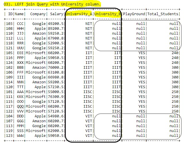
With Left join concept all the left table records will be printed (more than existing records also possible when multiple matches found in right or second table) +
matching records from right table will have proper values and non matching records from right table will have null values.

In the diagram University_A column have all the values available from Student_Table , in University_B column we have proper values for matching values(IIT, IIIT, IISC) and null will be applicable for non-matching values (NIT, VIT). If we select other columns from right table those column values will also be represented with null values for non-matching column values which we used in join condition.
Output:

O4). RIGHT JOIN:

#print("O4). RIGHT join Query with University column.")
sql_query="""
SELECT A.ID, A.Name, A.Company, A.Salary, 
A.University AS University_A, B.University AS University_B, 
B.PlayGround, B.Total_Students 
FROM Student_Table A 
RIGHT JOIN University_Table B
ON A.University = B.University
"""
spark.sql(sql_query).show()

Explanation: Here RIGHT JOIN can also called as RIGHT OUTER JOIN.

With RIGHT join concept all the right table records will be printed (more than existing records also possible when multiple matches found in left or other table) +
matching records from left table will have proper values and non matching records from left table will have null values.

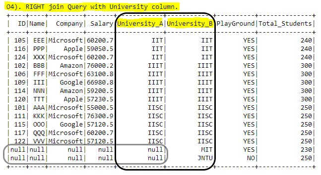
In the diagram University_B column have all the values available from University_Table , in University_A column we have proper values for matching values(IIT, IIIT, IISC) and null will be applicable for non-matching values (MIT, JNTU). If we select other columns from left table those column values will also be represented with null values for non-matching column values which we used in join condition. If we observe we have more records in output even though only 5 records in University_Table this is because one value in right table have multiple matches in left table.
Output:

O5). FULL OUTER JOIN:

#print("O5). FULL OUTER join Query with University column.")
sql_query="""
SELECT A.ID, A.Name, A.Company, A.Salary, 
A.University AS University_A, B.University AS University_B, 
B.PlayGround, B.Total_Students 
FROM Student_Table A 
FULL OUTER JOIN University_Table B
ON A.University = B.University 
"""
spark.sql(sql_query).show()

Explanation: Here FULL JOIN can also called as FULL OUTER JOIN.
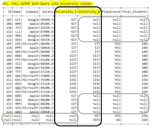
This will return all the values from left, right tables. For matching values in join condition will be assigned proper values and for non-matching values null will be assigned. If we observe the diagram FULL JOIN is nothing but LEFT JOIN + RIGHT JOIN.

In University_A column we can see NIT, VIT values and for these values in University_B or right table null will be assigned because of non-matching criteria.
Similar way in University_B column we can see MIT, JNTU values and for these values in University_A or left table null will be assigned because of non-matching criteria.

Output:

O6). CROSS JOIN:

#print("O6). Example for Cross Join Query")
#print("\nCount of Student_Table = ",student_dfps.count())
#print("\nCount of University_Table = ",university_dfps.count())
#print("\nCount(Student_Table) X Count(University_Table) = ",student_dfps.count() * university_dfps.count())

sql_query="""
SELECT A.ID, A.Name, A.Company, A.Salary, 
A.University AS University_A, B.University AS University_B, 
B.PlayGround, B.Total_Students 
FROM Student_Table A 
CROSS JOIN University_Table B
ORDER BY A.ID, B.University
"""
spark.sql(sql_query).show()

Explanation: Lets say we have 2 tables and we want to get the each row of first table with each row of second table combination CROSS JOIN will help us on this. We will get Cartesian product of rows from each table we used in join query. Here we wont use any matching criteria. In below Student_Table have 24 records, University_Table have 5 records. Now when we apply CROSS JOIN we will get 24 X 5 = 120 records in output.

If we observe the below output, for one ID (let say 101) from left table we have 5 records which contains all universities(IIIT, IISC, IIT, JNTU, MIT) from right table. Black box in the diagram have each student details from Student_Table, in Blue box the entire University_Table will be assigned.
Output:

P). Union, Union all, Except:

Joins concept used for clubbing multiple tables horizontally(combining columns) and UNION concepts used to club multiple tables vertically(combining rows). To apply UNION, UNION ALL, EXCEPT concepts we need make sure number of columns, order of the columns should be similar in both the tables.

UNION : Records will be clubbed and only distinct values will be printed.
UNION ALL : Records will be clubbed and all values will be printed(can have duplicates).
EXCEPT : Acts as Minus (-) and return the extra values in first table compared to second table.

P1). UNION:

#print("P1). UNION Example")
sql_query="""
SELECT University FROM Student_Table
UNION
SELECT University FROM University_Table
"""
spark.sql(sql_query).show()

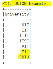
Explanation: To club multiple tables vertically (combining records) we use UNION statements. Here duplication is not allowed. Same number of columns and order also we need to maintain same for tables in UNION concepts.

In this example all the University values from Student_Table(NIT, IIT, IIIT, IISC, VIT) and values from University_Table(MIT, JNTU) combined in the output without duplication.

Output:

P2). UNION ALL:

#print("P2). UNION ALL Example")
sql_query="""
SELECT University FROM Student_Table
UNION ALL
SELECT University FROM University_Table
ORDER BY University
"""
spark.sql(sql_query).show()

Explanation: To club multiple tables vertically (combining records) we use UNION ALL statements. Here duplication is allowed. Same number of columns and order also we need to maintain same for tables in UNION ALL concepts.

In this example all the University values from Student_Table(NIT, IIT, IIIT, IISC, VIT) and values from University_Table(MIT, JNTU) combined in the output with duplication.
Output:

P3). EXCEPT:

#print("P3). EXCEPT Example")
sql_query="""
SELECT University FROM Student_Table
EXCEPT
SELECT University FROM University_Table
"""
spark.sql(sql_query).show()

Explanation: If we want to subtract the values from first select statement to second one we use this EXCEPT concept. Here duplication is not allowed. This will only give the extra records from first select statement compared to second select statement.
Output:

Q). Window functions:

Till now we seen Group By statements to apply aggregate functions to return single value for that group. By using Window functions we can able to partition the relevant records and we can do lot of customization within that partition such that we can achieve sorting the values within partition or assign some rank values by sorting the values or even we can able to get the running aggregation values for partition. Parition is nothing but grouping values based on some column(s).

In real time data analysis Window functions can play very important role to get the more insights about data. We can apply these window functions for partitions or for entire table level also. By using window functions we are going to create a new column which have outcome of the window function. In all window functions we will be using OVER() clause where we will be mentioning based on which column(s) table should be partitioned(i.e. Group By) and which columns has to be in sorting order(i.e. Order By). With these details new column will be created. We have couple of windows functions we are going to cover in this section.

ROW_NUMBER(): Assign a sequential value starts with 1 for each partition values.
RANK(): Assign the sequential value, if similar values found then rank will be same and for coming value rank will be skipped to those many similar values from original rank value.
DENSE_RANK(): Assign the sequential value, if similar values found then rank will be same and for coming value rank will not be skipped. Continuous rank will be applicable.
NTILE(): Distribute the entire table sorted records into specific number of equal groups or buckets.
LEAD(): will provide the value leading to given offset number of positions for current row.
LAG(): will provide the value lagging to given offset number of positions for current row.
Running aggregation functions in window functions(COUNT(), SUM(), AVG(), MIN(), MAX()): Returning aggregation value till that row from starting of partition.

Q1). ROW_NUMBER() Example-1 without Partition:

#print("Q1). Row_number based ID, without Partition.")
sql_query="""
SELECT ID, Name, Gender, Salary, Location, Company,
ROW_NUMBER() OVER(ORDER BY ID) AS RowNumber_by_ID
FROM Student_Table
"""

spark.sql(sql_query).show()

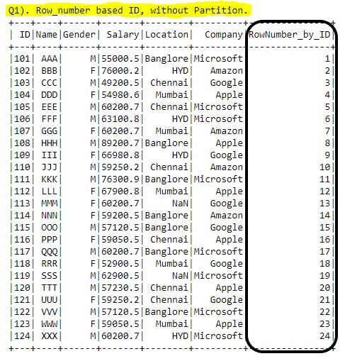
Explanation: ROW_NUMBER() is mainly used to create a new column with sequential number starting with 1 for entire table level or for each partition. In this example we are covering for entire table level(without any partition, next example we will cover for partition level). With ROW_NUMBER() function ORDER BY clause is mandatory to use.
In this example ROW_NUMBER() OVER(ORDER BY ID) AS RowNumber_by_ID after the ROW_NUMBER() function we have used OVER() clause where we have mentioned how the output format should be(GROUP BY, ORDER BY). For new column we are renaming with ALIAS keyword followed by new column name RowNumber_by_ID.
Output:

Q2). ROW_NUMBER() Example-2 with Partition:

#print("Q2). Row_number PARTITION BY Location ORDER BY Company.")
sql_query="""
SELECT ID, Name, Gender, Salary, Company, Location, 
ROW_NUMBER() OVER(PARTITION BY Location ORDER BY Company) AS RowNumber_Location_Company
FROM Student_Table
"""

spark.sql(sql_query).show()

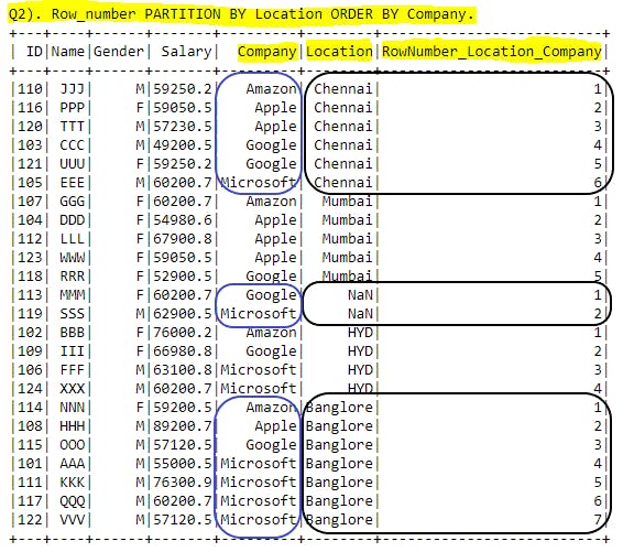
Explanation: Here ROW_NUMBER() OVER(PARTITION BY Location ORDER BY Company) AS RowNumber_Location_Company we have used PARTITION BY on top of Location column so that output will be grouped based on Location column and ORDER BY based on Company so that in each group of Location all available records will be sorted according to Company in ascending order(default order type). Now within each Partition we can able to see sequence numbers starting from 1. This sequence will be reset to 1 again for next partition.

In the output we could see that in Location column all similar values grouped together and in Company column all the available companies in that location will be sorted ascending order. Now the new column RowNumber_Location_Company has been created with sequential number for each Location. No duplicates found in within same group.
Output:

Q3). RANK:

#print("Q3). Rank function with PARTITION BY Company ORDER BY Salary.")

sql_query="""
SELECT ID, Name, Gender, Location, Company, Salary,
RANK() OVER(PARTITION BY Company ORDER BY Salary DESC) AS Rank_Salary_Company
FROM Student_Table
"""

spark.sql(sql_query).show()

Explanation: By using RANK() function we are grouping(Partition) the records based on Company column and sorting(ORDER BY ) the Salary in descending order and creating a new Rank_Salary_Company column.

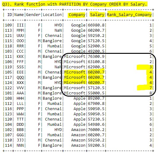
In new column if we observe for Microsoft company Salary details are in descending order and forID = 105, 117, 124 we have same salaries highlighted in screenshot. If we have similar values in RANK() function it will assign the same rank for similar records but coming ID=122 rank has been assigned as 7. Because number of similar values =3 and rank for those similar values =4 so now RANK() function will add these numbers and assign the rank for up coming records 3+4=7. Same we can observe for ID=122 rank as 7.

RANK() function will assign the same sequence number for similar values and skip the sequence number till general sequence number(without skipping and without repetition) and assign that number. i.e. whatever we get after applying ROW_NUMBER() we will get the same if we have similar record values.

Output:

Q4). DENSE_RANK():

#print("Q4). DENSE_RANK function with PARTITION BY Company ORDER BY Salary.")
sql_query="""
SELECT ID, Name, Gender, Location, Company, Salary,
DENSE_RANK() OVER(PARTITION BY Company ORDER BY Salary DESC) AS DENSE_Rank_Salary_Company
FROM Student_Table
"""

spark.sql(sql_query).show()

Explanation: By using DENSE_RANK() function we are grouping(Partition) the records based on Company column and sorting(ORDER BY ) the Salary in descending order and creating a new DENSE_Rank_Salary_Company column.

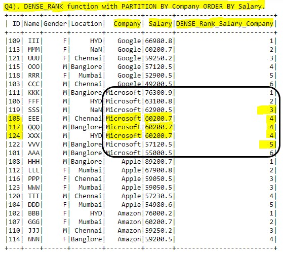
In new column if we observe for Microsoft company Salary details are in descending order and forID = 105, 117, 124 we have same salaries highlighted in screenshot. If we have similar values in DENSE_RANK() function it will assign the same rank for similar records but for coming ID=122 DENSE_RANK has been assigned as 4. Here in DENSE_RANK() sequence number will not get skipped and after all matching records completed without breaking sequence will be continued. Same we can observe for ID=122 DENSE_RANK=5.

DENSE_RANK() function will assign the same sequence number for similar values and won't skip the sequence number for upcoming records and sequence will be continued.

Output:

Q5). ROW_NUMBER, RANK, DENSE_RANK in single output:

#print("Q5).ROW_NUMBER, RANK, DENSE_RANK in single output:")

sql_query="""
SELECT ID, Name, Gender, Location, Company, Salary,
ROW_NUMBER() OVER(PARTITION BY Company ORDER BY Salary DESC) AS ROW_NUMBER,
RANK() OVER(PARTITION BY Company ORDER BY Salary DESC) AS RANK,
DENSE_RANK() OVER(PARTITION BY Company ORDER BY Salary DESC) AS DENSE_RANK
FROM Student_Table
"""

spark.sql(sql_query).show()

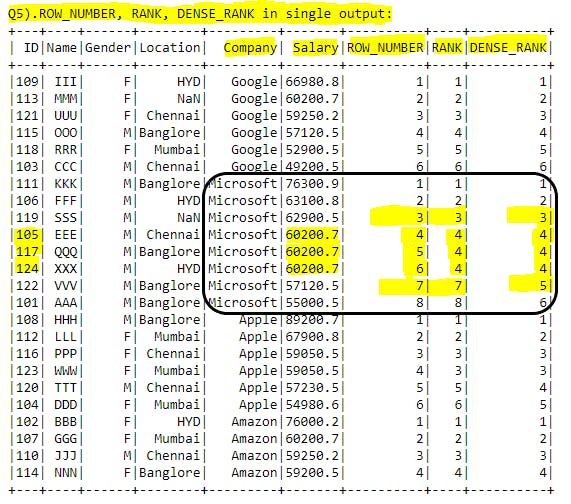
Explanation: Just for comparison purpose I've added ROW_NUMBER, RANK, DENSE_RANK functions in single query. By seeing this example we can easily understand that
ROW_NUMBER is sequence number without any breaks or duplicates.
RANK will have duplicates when data matches and skip the upcoming records ranking.
DENSE_RANK will have duplicates when data matches and wont skip the upcoming records ranking.
Output:

Q6). NTILE:

#print("Q6).Distribute ID's into NTILE(5) equal buckets.")
sql_query="""
SELECT ID, Location,
NTILE(5) OVER(ORDER BY ID) AS NTILE_on_ID
FROM Student_Table
"""

spark.sql(sql_query).show()

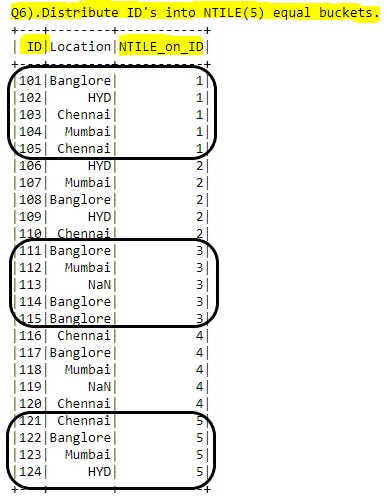
Explanation: To apply NTILE() function at least one column should have sorted data. Lets say if we want to divide entire table rows into some equal buckets we can use this function. Simply that we are creating a new column by assigning bucket number for each row. We are mentioning in NTILE(5) function itself how many buckets we are going to place for all records. Based on this number(5) record count of table will divide and group those many number of records to each bucket. Sometimes for last bucket we may see less records than other buckets because of record count dividable by given number of buckets might not give always zero(0) as a reminder.
Here we have total of 24 records and number of buckets are 5 with this we will definately get only 4 records in last bucket.
Output:

Q7). LEAD:

#print("Q7).Lead function on Salary column by offset = 2.")

sql_query="""
SELECT ID, Location, Company, Salary, 
LEAD(Salary,2) OVER(ORDER BY ID) AS Lead_2_Salary
FROM Student_Table
"""

spark.sql(sql_query).show()

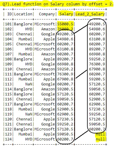
Explanation: LEAD() function is used to create a new column based on existing column values by leading the given number of offset records to the existing column values. Here offset number is important because those many number of records will be skipped first and assigning values after the offset position. Similar way in new column end of the records will have offset number to null values because there will not be any values to be assigned. Simply after the offset position entire column value will be copied and at the end null will be replaced.
Here LEAD(Salary, 2) the column we are going to apply this function is Salary and offset is 2 so first 2 record data skipped(wont be copied) and rest of the values will be copied to new column. In new column 2 records have null values.
Output:

Q8). LAG:

#print("Q8).Lag function on Salary column by offset = 3.")

sql_query="""
SELECT ID, Location, Company, Salary, 
LAG(Salary,3) OVER(ORDER BY ID) AS Lag_3_Salary
FROM Student_Table
"""

spark.sql(sql_query).show()

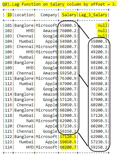
Explanation: LAG() function is used to create a new column based on existing column values by lagging the given number of offset records to the existing column values. Here offset number is important because those many number of records will be replaced as null in new column and then rest of the data will be copied into new column after that offset. Simply with given offset number of records in new column will be replaced with null then data will be copied to new column from after offset position.
Here LAG(Salary, 3) the column we are going to apply this function is Salary and offset is 3 so first 3 records in new column will be replaced as null and then entire data will be copied to new column. But for last given offset number of records in Salary values wont be copied to new column because there are no records in entire table and those many offset number of values will be missed to copy.
Output:

Q9). Running aggregation functions in window functions(COUNT(), SUM(), AVG(), MIN(), MAX()):

#print("Q9).Running Total example on Salary Column partition by Company.")

sql_query="""
SELECT ID, Location, Company, Salary, 
SUM(ROUND(SALARY)) OVER (PARTITION BY COMPANY ORDER BY SALARY) AS Running_Total
FROM Student_Table
"""

spark.sql(sql_query).show()

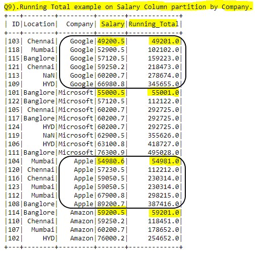
Explanation: In running aggregation functions we can use all aggregation functions we already used in earlier sections. Here in this example we are using SUM() for running aggregation i.e. we call it as running total. This will give the sum of given column till current row. It will calculate for every record in given partition. Value will get reset to new partition as first record value in that partition.
In this example we have used Salary column for running total with company as partition. Lets say for Google company first row will be same as existing value, in second row value will be assigned as sum of first row, second row. Similarly for 3rd row value be calculated as sum of 1st, 2nd, 3rd rows values. For new partition Microsoft the process will start again in same way.
Output:

Conclusion:

I hope you have learned SQL concepts with simple examples.
Happy Learning...!!

1.End.jpg

Python SQL spark Data Science data analysis

SQL + Python + Spark for Data Science

Table of contents

Table of Content:

Prerequisites:

A). Pyspark Connection - skip this section:

B). Create dataframe by reading files and datatype conversion - skip this section:

B1). Create Student dataframe and define datatypes in pyspark:

B2). Create University dataframe and define datatypes in pyspark:

B3). Create Company dataframe and define datatypes in pyspark:

B4). Create Year_Month_Day dataframe and define datatypes in pyspark:

C). Create TempView(Table), Data overview and size(count)- skip this section:

C1). Student_Table Schema, Row count, Data Overview:

C2). Student_Table Schema, Row count, Data Overview:

C3). Company_Table Schema, Row count, Data Overview:

C4). Year_Month_Day_Table Schema, Row count, Data Overview:

D). Select statement ( * , AS, LIMIT, COUNT(), DISTINCT ):

D1). Select only few columns + LIMIT:

D2). Select all the columns + LIMIT:

D3). Alias names for columns :

D4). Counting number of records:

D5). Select some random text:

D6). Distinct in select statement:

E). Where clause(BETWEEN, LIKE, IN, AND, OR):

E1). WHERE clause:

E2). WHERE clause + BETWEEN:

E3). WHERE clause + LIKE:

E4). WHERE clause + IN:

E5). WHERE clause + AND:

E6). WHERE clause + OR:

F). Order By:

F1). ORDER BY + ASC:

F2). ORDER BY + DESC:

G). Upper(), Lower(), Length() functions:

H). Concatenation(||) + BooleanExpression + TRIM() functions:

H1). Concatenation (||):

H2). Boolean Expression:

H3). TRIM() function:

I). SUBSTRING() + REPLACE() + POSITION() functions:

I1). SUBSTRING() function:

I2). REPLACE() function:

I3). POSITION() function:

J). Aggregation functions:

J1). COUNT() function:

J2). MAX() function:

J3). MIN() function:

J4). SUM(), AVG() functions:

K). GROUP BY + HAVING clauses:

K1). GROUP BY Example-1:

K2). GROUP BY Example-2:

K3). GROUP BY + Having:

L). Sub Queries:

L1). Subquery Example-1:

M). Correlated sub queries:

M1). Correlated sub query Example-1:

N). Case statement:

N1). Case Statement Example-1:

O). Joins (INNER, LEFT, RIGHT, FULL, CROSS):

O1). Joins concept overview with Example-1:

O2). INNER JOIN:

O3). LEFT JOIN:

O4). RIGHT JOIN:

O5). FULL OUTER JOIN:

O6). CROSS JOIN:

P). Union, Union all, Except:

P1). UNION:

P2). UNION ALL:

P3). EXCEPT:

Q). Window functions:

Q1). ROW_NUMBER() Example-1 without Partition:

Q2). ROW_NUMBER() Example-2 with Partition:

Q3). RANK:

Q4). DENSE_RANK():

Q5). ROW_NUMBER, RANK, DENSE_RANK in single output:

Q6). NTILE:

Q7). LEAD:

Q8). LAG:

Q9). Running aggregation functions in window functions(COUNT(), SUM(), AVG(), MIN(), MAX()):

Conclusion:

D). Select statement ( `*` , AS, LIMIT, COUNT(), DISTINCT ):