Pandas - Python for Data Science
Pandas Series, DataFrame and multiple operations on 2D data
Table of contents
- Table of Content:
- Prerequisites:
- Introduction:
- A). Import required packages:
- B). Series in Pandas:
- C). DataFrame in Pandas:
- D). DataFrame - General functions:
- E). DataFrame Columns Manipulation - Select, Create, Rename, Drop:
- F). DataFrame Rows Manipulation - Select, Create, Rename, Drop:
- F1). Sample dataframe for reference in this section:
- F2). Select single row using loc[] :
- F3). Selecting multiple rows using loc[]:
- F4). Selecting few rows with few columns using loc[]:
- F5). Select single row using iloc[] :
- F6). Selecting multiple rows using iloc[]:
- F7). Selecting few rows and few columns using iloc[]:
- F8). Create a new row using loc[]:
- F9). Create a new row using iloc[]:
- F10). Drop the row in dataframe:
- F11). Rename row index name in dataframe:
- F12). Conditional selection of dataframe:
- F13). Conditional selection-2 of dataframe:
- F14). Conditional selection-3 of dataframe:
- F15). Conditional selection-4 of dataframe:
- G). Missing data Manipulations:
- G1). Sample dataframe with missing data :
- G2). isnull() function to get boolean matrix:
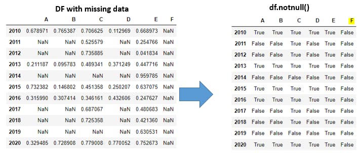
- G3). notnull() function to get boolean matrix:
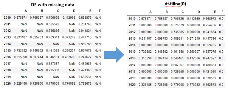
- G4). fillna(value, method=[ffill,bfill], axis=[0,1]) function-1:
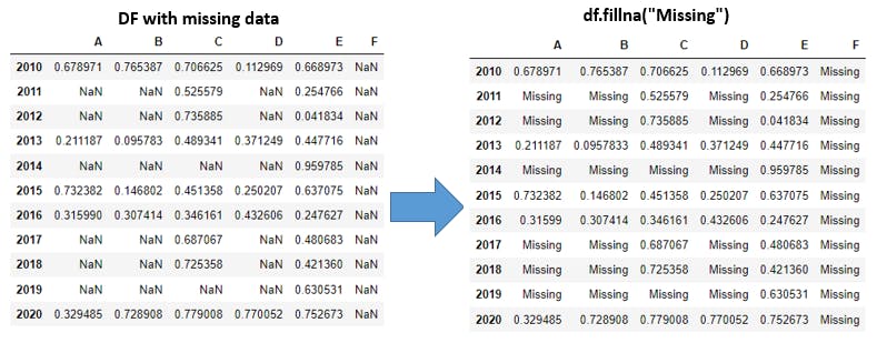
- G5). fillna(value, method=[ffill,bfill], axis=[0,1]) function-2:
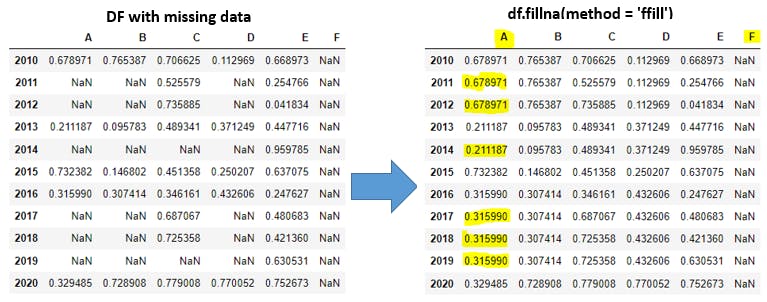
- G6). fillna(value, method=[ffill,bfill], axis=[0,1]) function-3: (forward filling vertically):
- G7). fillna(value, method=[ffill,bfill], axis=[0,1]) function-4: (forward filling horizontally):
- G8). fillna(value, method=[ffill,bfill], axis=[0,1]) function-5: (backward filling vertically):
- G9). fillna(value, method=[ffill,bfill], axis=[0,1]) function-6: (backward filling horizontally):
- G10). Replace missing data for all columns:
- G11). Replace missing data only for few columns:
- G12). dropna(axis=[0,1], how=[any,all], thresh) Ex-1:
- G13). dropna(axis=[0,1], how=[any,all], thresh) Ex-2:
- G14). dropna(axis=[0,1], how=[any,all], thresh) Ex-3:
- G15). dropna(axis=[0,1], how=[any,all], thresh) Ex-4:
- G16). dropna(axis=[0,1], how=[any,all], thresh) Ex-5:
- G17). dropna(axis=[0,1], how=[any,all], thresh) Ex-6:
- G18). dropna(axis=[0,1], how=[any,all], thresh) Ex-7:
- G19). dropna(axis=[0,1], how=[any,all], thresh) Ex-8:
- G20). dropna(axis=[0,1], how=[any,all], thresh) Ex-9:
- H). Group by in Dataframes:
- I). Combine multiple dataframes:
- I1). Sample Dataframes:
- I2). merge(df1, df2, how='inner') Ex-1: You can skip this example:
- I3). merge(df1, df2, how='inner') Ex-2:
- I4). merge(df1, df2, how='left', on=['A', 'D']):
- I5). merge(df1, df2, how='right', on=['A', 'D']):
- I6). merge(df1, df2, how='outer', on=['A', 'D']):
- I7). join() function:
- I8). concat([df1, df2, df3]):
- I). concat([df1, df2, df3] axis=0):
- Conclusion:
Table of Content:
In this Pandas tutorial, we will be learning below concepts.
- Prerequisites, Introduction
- A). Import required packages:
- B). Series in Pandas:
- C). DataFrame in Pandas:
- D). DataFrame - General functions:
- E). DataFrame Columns Manipulation - Select, Create, Rename, Drop:
- F). DataFrame Rows Manipulation - Select, Create, Rename, Drop:
- G). Missing data Manipulations:
- H). Group by in Dataframes:
- I). Combine multiple dataframes - Merge, Join, Combine:
- Conclusion
Prerequisites:
Pandas concepts are very easy to learn and apply in the real world applications.
Ex: If we understand our high school marks(grade) card with subjects along with marks in each subject
this example is more than enough to digest the entire Pandas concepts.
Introduction:
- Pandas is used for Processing (load, manipulate, prepare, model, and analyze) the given data. Pandas is built on top of the Numpy package so Numpy is required to work with Pandas.
- Pandas has 2 data structures for processing the data.
-
Series: is a one-dimensional array that is capable of storing various data types. -
DataFrame: is a two-dimensional array with labeled axes (rows and columns).
-
A). Import required packages:
import numpy as np
import pandas as pd
Explanation: import key word is used to import the required package into our code. as keyword is used for giving alias name for given package. numpy is the numerical python package used to create numerical arrays in this tutorial.
Example: pandas is the package and pd is the alias name or short name for pandas.
B). Series in Pandas:
- Series is a 1-dimensional array which capable of storing various data types(Integers, strings, floating point numbers, Python objects).
- The row labels of series are called the index.
- Series cannot contain multiple columns. It will be having only one column.
- Lets explore some of the examples of series in Pandas.
B1). Create Series from Python Dictionary
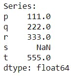
dict1 = {'p':111, 'q':222, 'r':333, 's':np.NaN, 't':555}
s = pd.Series(dict1)
print(s)
Explanation: Here p,q,r,s,t are called indexes. pd.Series() is used to create Pandas series. Note: S in Series() is capital.
Output:
B2). Series from Scalar value
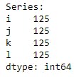
s = pd.Series(125, index=['i','j','k','l'])
print(s)
Explanation: Here all indexes 'i','j','k','l' will be having same value 125.
Output:
B3). Series from Numpy array
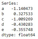
s = pd.Series(np.random.randn(5), index=['a','b','c','d','e'])
print(s)
Explanation: np.random.randn(5) will be creating 5 random numbers.
Output:
B4). Series Functionalities
dict1 = {'p':111, 'q':222, 'r':333, 's':np.NaN, 't':555}
s = pd.Series(dict1)
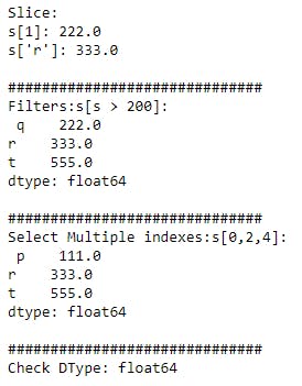
print("Slice:\n s[1]:",s[1])
print("s['r']:",s['r'])

print("\n##############################")
print("Filters:s[s > 200]:\n", s[s > 200])

print("\n##############################")
print("Select Multiple indexes:s[0,2,4]:\n", s[[0,2,4]])

print("\n##############################")
print("Check DType:", s.dtype)
Explanation: We can apply Slice, filters, selecting particular indexes, check for data type of the series. s[1] is for printing the value at index 1 whereas index starts at 0. s[s > 200] is used for filtering the data which are graterthan 200. s[[0,2,4]] with this we can select multiple indexed value at single step. s.dtype is for checking Series data type.
Output:
C). DataFrame in Pandas:
- DataFrame is a two-dimensional array with labeled axes (rows and columns).
- DataFrame is like Structured table or Excel file.
- Lets explore some of the examples of Dataframe in Pandas.
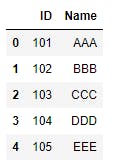
C1). Dataframe from Python Dictionary
dict1 = {"ID":[101,102,103,104,105], "Name":['AAA','BBB','CCC','DDD','EEE']}
df = pd.DataFrame(dict1)
df
Explanation: Here ID, Name are the columns and index will be auto generated at left side.
Output:
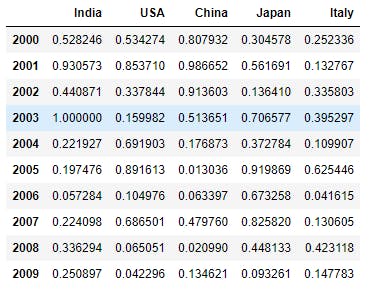
C2). Dataframe from Numpy n-d array:
a = np.array(np.random.rand(10,5))
df = pd.DataFrame(a, index = [np.arange(2000,2010)], columns = ['India', 'USA', 'China', 'Japan', 'Italy'])
df
Explanation: a is for tabular data, np.arange() used for index, columns used for columns header.
Output:
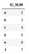
C3). DataFrame from List:
l1 = [2,3,4,5,6,7]
df = pd.DataFrame(l1, index = ['a','b','c','d','e','f'], columns = ['ID_NUM'])
df
Explanation: l1 for Data. 'a','b','c','d','e','f' are the index values and ID_NUM is the column header.
Output:
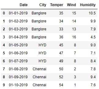
C4). DataFrame from CSV file:
df = pd.read_csv("Pandas_Blog.csv")
df
Explanation: read_csv function used for reading CSV files from local machine. Entire data in csv file will be accessable from Pnadas dataframe df. You can download this sample CSV file from here.
Output:
D). DataFrame - General functions:
Most of the time as a Data Analyst or Data Scientist we will be dealing with DataFrames very frequently. Lets explore some of the basic functionalities applied on top of DataFrame level. Before that lets use the sample dataframe for rest of the tutorials so that it will be very useful to apply our thoughts for any dataframe we come across.
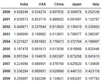
D1). Sample DataFrame for rest of the tutorials.
a = np.array(np.random.rand(10,5))
df = pd.DataFrame(a, index = [np.arange(2000,2010)], columns = ['India', 'USA', 'China', 'Japan', 'Italy'])
df
Explanation: This example we already seen in our examples. Please be noted that you may get different values in the table as we are using random function here. Due to this we may get different values than these values it will get change system to system.
Output:
D2). info() function:
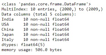
df.info()
Explanation: info() function will be used for giving overall information about dataframe like number of columns, number of rows(records), column names and their data types, each column contains null values or non-null values.
With info() function we can get entire high level understanding on the dataframe.
Output:
D3). describe() function:
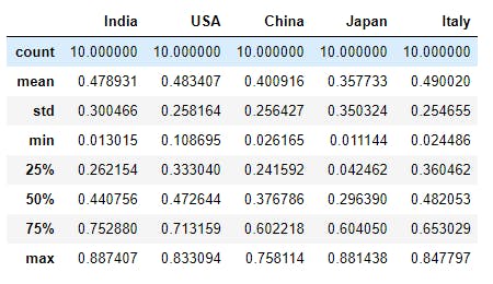
df.describe()
Explanation: describe() function used for checking the statistical information about all numerical columns data. It will show us the min, max, mean, 25%, 50%, 75% of the numerical columns.
Output:
D4). count() function:
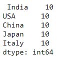
df.count()
Explanation: count()function will show us in each column how many non-null records (non-missing or proper values) are exists. Here in each column we are having 10 records without any missing data.
Output:
D5). columns attribute:
df.columns
Explanation: columns will be printing the list of columns in the dataframe. Note: We shouldn't use () with this attribute.
Output:

D6). index attribute:
df.index
Explanation: index attribute will printout the indexes available for the dataframe.
In the output levels is the user defined index and labels is the existing default index for the dataframe.
Output:

D7). shape attribute:
df.shape
Explanation: shape will print the number of rows, number of columns in the dataframe. It is like dimensions for the matrix. Ex: (rows, columns) = (10,5)
Output:

D8). dtypes attribute:
df.dtypes
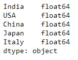
Explanation: dtypes will print the each column and corresponding data type of the column side by side.
Output:
D9). head() function:
df.head(3)
Explanation: head() function will print the first or top n records in the dataframe. Here n=3. First 3 rows with all the columns will be shown.
Output:

D10). tail() function :
df.tail(3)
Explanation: tail() function will print the last or bottom n records in the dataframe. Here n=3. Last 3 rows with all the columns will be shown.
Output:

D11). sample() function :
df.sample(3)
Explanation: sample() will print n random rows from the dataframe.
Output:

E). DataFrame Columns Manipulation - Select, Create, Rename, Drop:
In the Pandas dataframe we mainly have rows and columns. In this section we starts with columns manupulations like how to ( Select, Create, Rename, Drop ) particular columns in dataframe. In general while dealing with dataframe rows and columns we need to specify axis value to 1 or 0.
axis = 0 for rows , axis = 1 for columns in the dataframe.
E1). Sample dataframe for this Columns Manipulation section:
a = np.array(np.random.rand(10,5))
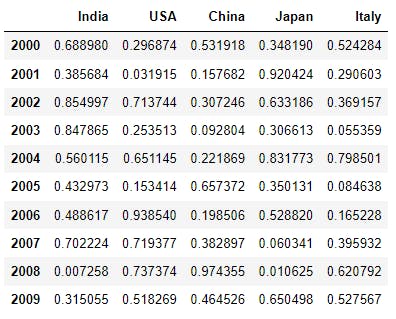
df = pd.DataFrame(a, index = [np.arange(2000,2010)], columns = ['India', 'USA', 'China', 'Japan', 'Italy'])
df
Explanation: This example we already seen in our examples. Please be noted that you may get different values in the table as we are using random function here. Due to this we may get different values than these values it will get change system to system.
Output:
E2). Selecting single column from dataframe:
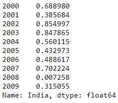
df['India']
Explanation: From the dataframe df we are selecting one single column India. We can cross check this output with our main dataframe in E1 section.
Output:
E3). Check the datatype of particular column:
type(df['India'])
Explanation: df['India'] code will select the India column. type() function will provide the datatype of India column.
Output:

E4). Selecting multiple columns from dataframe:
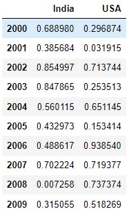
df[['India', 'USA']]
Explanation: From the dataframe df we are selecting multiple columns India, USA. Here we have to pass the required multiple columns in the form of List like ['India', 'USA']. We can cross check this output with our main dataframe in E1 section.
Output:
E5). Create new column to the dataframe:
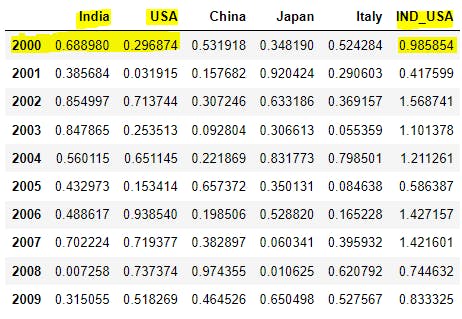
df['IND_USA'] = df['India'] + df['USA']
df
Explanation: Here we are creating new column called IND_USA and in r.h.s we have to assign the value. Here we are adding the values of each row from India, USA and assigning to IND_USA column.
Ex: For 2000 year, India = 0.688980 and USA = 0.296874. Now IND_USA = 0.985854.
Output:
E6). Rename the dataframe column:
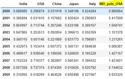
df = df.rename(columns={'IND_USA':'IND_puls_USA'})
df
Explanation: rename() function help us to rename the given column. Inside this function we have to pass the columns keyword with key-value paired. Here Key = Existing column name, Value = New Proposed column name.
Ex: Here IND_USA is existing column name and IND_puls_USA is new column name.
Output:
E7). Dropping existing column:
df = df.drop('IND_puls_USA', axis=1)
df
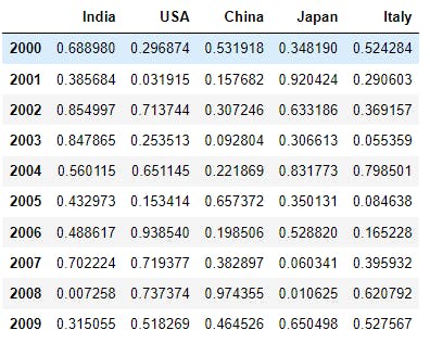
Explanation: drop function will help us to remove or delete the existing column. Inside function we are passing the column name IND_puls_USA. With axis=1 we are informing the compiler to remove the column but not the row.
Note: If we skip the axis=1 syntax, if any row index is having name as IND_puls_USA then that row will be deleted. To skip that row deletion, we are giving axis=1 to delete the column which name is IND_puls_USA. After deletion we will not get the data back, so have to be cautious while using drop() function. After deletion of IND_puls_USA column, our dataframe looks like below.
Output:
F). DataFrame Rows Manipulation - Select, Create, Rename, Drop:
In this section we will learn about Rows manupulations like how to ( Select, Create, Rename, Drop ) particular rows in dataframe. In general while dealing with dataframe rows and columns we need to specify axis value to 1 or 0. axis = 0 for rows , axis = 1 for columns in the dataframe.
Accessing rows from dataframe can be done in these 2 ways by using loc() and iloc() functions.
axis = 0for rows selection,axis = 1for columns selection. in the row selection again we have 2 parameters as below:
loc()- used when we know index name for a perticular row.iloc()- used when we dont know the name of index, but we know index order value
F1). Sample dataframe for reference in this section:
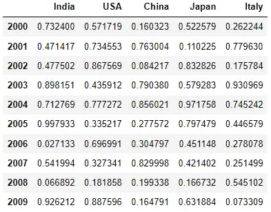
a = np.array(np.random.rand(10,5))
df = pd.DataFrame(a, index = np.arange(2000,2010), columns = ['India', 'USA', 'China', 'Japan', 'Italy'])
df
Output:
df.index
Explanation: Here if we observe loc() can be applied on row index name or levels like 2000, 2001, ..., 2009 and iloc() can be applied on row index numbers or labels like 0, 1, ...,9.
Output:

F2). Select single row using loc[] :
df.loc[2005]

or

df.iloc[5]
Explanation: From dataframe we are selecting row which is having index name as 2005. It is similar to selecting 5 index number using iloc[5]. Because we know there is a 2005 index name, so that we can directly use loc[2005]. If we are not sure on index name then we can use index number using iloc[5].
Output: 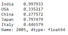
F3). Selecting multiple rows using loc[]:
df.loc[[2005, 2007]]
Explanation: For multiple row selection we have to give the list with required index names to loc[]. By default we will get all the columns in the given row.
Output:

F4). Selecting few rows with few columns using loc[]:
df.loc[[2005, 2007], ['India', 'USA']]
Explanation: Here we are providing 2 lists to the loc[]. First one is the list of index names we require and second list for list of column names we require to print. These 2 lists can be separated by ,.
Output:

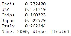
F5). Select single row using iloc[] :
df.iloc[0]
Explanation: Here we are selecting 0 indexed row or 2000 index name row with all columns.
Output:
F6). Selecting multiple rows using iloc[]:
df.iloc[[0,2]]
Explanation: Here we are giving list of index numbers which we want to display. This will print index 0,2 rows with all columns.
Output:

F7). Selecting few rows and few columns using iloc[]:
df.iloc[[0, 2], [0,1]]
Explanation: Here using iloc[] we are printing 0,2 rows and 0,1 columns from the dataframe df.
Output: 
F8). Create a new row using loc[]:
df.loc[2010] = np.random.rand(5)
df
Explanation: Here we dont have index named 2010 till now and creating 2010 index name with 5 random numbers.
Output: 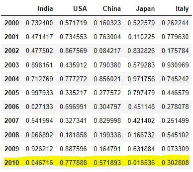
F9). Create a new row using iloc[]:
df.iloc[10] = np.random.rand(5)
df
Explanation: Here we are recreating 2010 row using 5 random numbers by using index number 10 with help of iloc[]. Values in 10 index number will get changed to previous example.
Output: 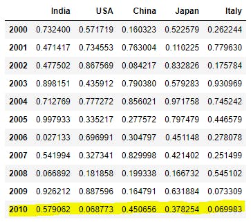
F10). Drop the row in dataframe:
df = df.drop(2010)
df
Explanation: Here we haven't specified the axis=0. By default rows will get dropped with drop() function. We will not be able to see the 2010 record.
Output: 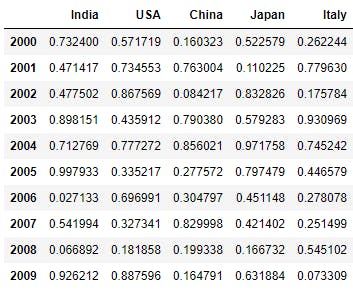
F11). Rename row index name in dataframe:
df = df.rename(index={2009:20009})
df

#renamed back to normal with below commented lines.
#df = df.rename(index={20009:2009})
Explanation: Here we are renaming 2009 index name to 20009 with rename() function. For simplicity purpose I've reverted the changes for upcoming sections.
Output: 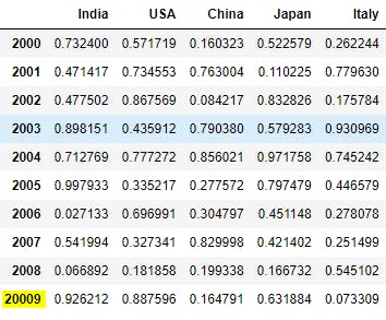
F12). Conditional selection of dataframe:
df>0.3
Explanation: Conditional selection will print us the boolean matrix of dataframe with given condition. Here df>0.3 says all values matches this condition will become true and remaining all cells become False. This matrix can be utilized in many places to filter out the data using conditions.
Output: 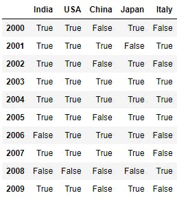
F13). Conditional selection-2 of dataframe:
df[df>0.3]
Explanation: Here we are passing conditional selection to dataframe level so that all true values will only be shown and remaining values will be printed as Nan i.e. Not a Number. First df>0.3 will be calculated and boolean matrix will be applied to dataframe df.
Output: 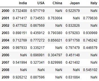
F14). Conditional selection-3 of dataframe:
df[df['India']>0.3]
Explanation: Here we are telling if India column is having greater than 0.3 value then print all of those rows will all columns combination.
Ex: Here 2006 index name in India column is having 0.027133 and it is not true so this 2006 row will not be printed in output.
Output: 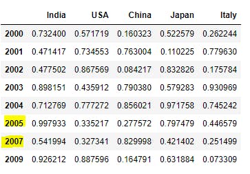
F15). Conditional selection-4 of dataframe:
df[df['India']>0.3][['India', 'USA']]
Explanation: On top of above example here we are selecting few columns only by proving list of columns we require at the end as [['India', 'USA']].
Output: 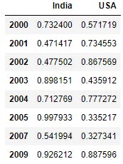
G). Missing data Manipulations:
Some times the data we are dealing might be having missing values. These missing data can be represented in Pandas as NaN i.e. Not a Number.
Ex: Let say we are collecting user information for some social media platform. Some users will not provide the address or personal information we are treated as optional fields. These missing fields can be considered as Missing Data.
Nan is a numpy object and None is None type object. Numpy objects better in performance than any other type. So Pandas mainly use NaN over the None to improve performance. This is from Numpy package(np.nan), widely used in numpy arrays , Pandas Series and Dataframes.
isnull():Generate a boolean mask indicating missing values.notnull(): Generate a boolean mask indicating proper values.fillna(): we can replaceNANwith a scalar value or text.dropna(): used to drop the row or column if it have missing data.
G1). Sample dataframe with missing data :
df = pd.DataFrame(np.random.rand(5,4), index =[2010, 2013, 2015, 2016, 2020], columns = 'A B C D'.split())
df = df.reindex(np.arange(2010,2021))
df['C'] = np.random.rand(11)
df.loc[2014] = np.nan
df.loc[2019] = np.nan
df['E'] = np.random.rand(11)
df['F'] = np.nan
df
Explanation: This is a sample dataframe for this section. Step1: Create dataframe with 5 rows(2010, 2013, 2015, 2016, 2020) and 4 columns(A, B, C, D) with random numbers.
Step2: Creating rows with index names from 2010 to 2021 and new rows can have missng data by default.
Step3: Creating new column C and filling with random numbers.
Step4, 5: Replacing 2014 and 2019 rows in NaN values.
Step6,7: Creating new columns E, F and assigning values.
Output: 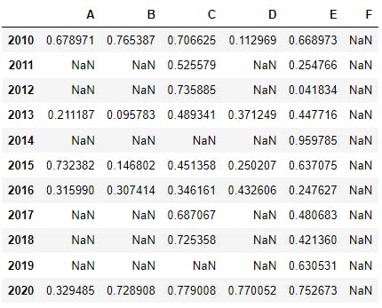
G2). isnull() function to get boolean matrix:
df.isnull()
Explanation: isnull() function will provide the boolean matrix of the given dataframe. It will check the data in each cell and if it found NaN then it will print True else it will print False.
Ex: Entire F column is having NaN. So in boolean matrix F column will contain only True values.
Output: 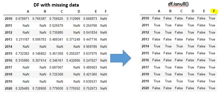
G3). notnull() function to get boolean matrix:
df.notnull()
Explanation: notnull() function is inverse of isnull() function and it will provide the boolean matrix of the given dataframe. It will check the data in each cell and if it found NaN then it will print False else it will print True.
Ex: Entire F column is having NaN. So in boolean matrix F column will contain only False values.
Output:
G4). fillna(value, method=[ffill,bfill], axis=[0,1]) function-1:
df.fillna(0)
Explanation: fillna() function to replace the missing data with given value. We have much control on how to fill the missing data with method=[ffill,bfill]. Here ffill means forward fill, bfill means backward fill with given value.
axis=[0,1] will represent horizontal(axis=1) or vertical(axis=0) axes to apply ffill or bfill parameters with given value. In this example we are simply assigning 0 to the missing data.
Output:
G5). fillna(value, method=[ffill,bfill], axis=[0,1]) function-2:
df.fillna("Missing")
Explanation: With fillna() function we are filling all missing values with text called Missing.
Output:
G6). fillna(value, method=[ffill,bfill], axis=[0,1]) function-3: (forward filling vertically):
df.fillna(method = 'ffill')

#forward filling vertically
Explanation: Here we have not provided the value and axis parameters. By default axis=0 which means vertically and ffill means forward filling will be applicable.
Ex: In column A index 2011, 2012 are missing so 2010 data will be copied forward filling in vertical(all rows) manner. Similarly 2013 data will be copied to 2014. Same way 2016 data will be copied to 2017, 2018, 2019 indexes in all the columns.
In Column F all rows are missing so no data has been taken forward in vertically to modify the missing data because first row(2010) in F column is also missing.
Output:
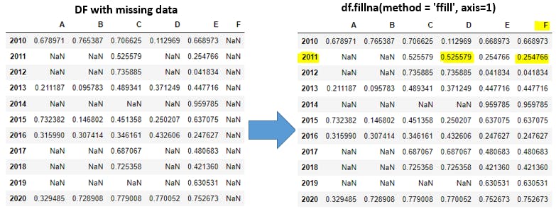
G7). fillna(value, method=[ffill,bfill], axis=[0,1]) function-4: (forward filling horizontally):
df.fillna(method = 'ffill', axis=1)

# forward filling horizontally
Explanation: axis=1 means horizontally forward fill will takes place.
Ex: In 2011 row D column will get replaced with Ccolumn data. Similarly F column will get replaced with Ecolumn data. A,B columns in 2011 row will remain same as missing because no prior columns there to take place of forward filling in horizontal manner.
If we observe columns E, F are having same data because all rows from column E copied to column F.
Output:
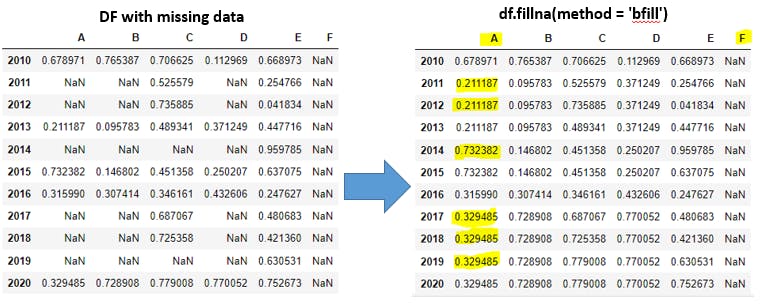
G8). fillna(value, method=[ffill,bfill], axis=[0,1]) function-5: (backward filling vertically):
df.fillna(method = 'bfill')

# backward filling vertically
Explanation: Here we have not provided the value and axis parameters. By default axis=0 which means vertically and bfill means backward filling will be applicable.
Ex: In column A index 2011, 2012 are missing so 2013 data will be copied backward filling in vertical(all rows) manner. Similarly 2015 data will be copied to 2014. Same way 2020 data will be copied to 2017, 2018, 2019 indexes in all the columns.
In Column F all rows are missing so no data has been taken backward in vertically to modify the missing data because last row(2020) in F column is also missing.
Output:
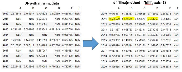
G9). fillna(value, method=[ffill,bfill], axis=[0,1]) function-6: (backward filling horizontally):
df.fillna(method = 'bfill', axis=1)

# backward filling horizontally
Explanation: axis=1 means horizontally backward fill will takes place.
Ex: In 2011 row D column will get replaced with Ecolumn data. Similarly A, B columns will get replaced with C column data. F column will remain have missing data as no other column existis right side to F column.
Output:
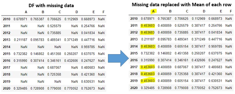
G10). Replace missing data for all columns:
df.fillna(df.mean())
Explanation: Within fillna() function we are using mean()function to findout the mean or average value in each row and filling the missing values.
EX: Lets see the mean value in column A with non missing values. The same mean value will be copied into all missing records in column A. Same will repeted for all columns missing data. Column F will remain same because all records in column F are missing.
Note: instead of mean() function, we can use any of the aggregation functions like sum(), min(), max(), prod(), std() functions. This task is very important in all the real time projects as data in real world will be having missing data and we need to replace those missing cells with proper data.
Output:

G11). Replace missing data only for few columns:
df.fillna(df.mean() ['B':'C'])
Explanation: Here we are only filling the mean() value in columns B, C. Rest of the columns will be having missing data.
Output: 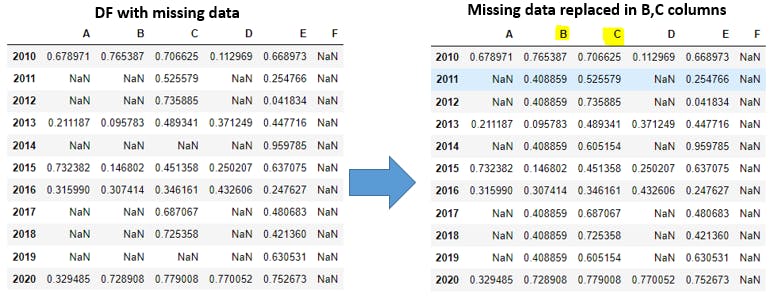
G12). dropna(axis=[0,1], how=[any,all], thresh) Ex-1:
df
Explanation: This section is for sample dataframe with missing data. dropna() function is useful when we want to remove the missing data in terms of rows and columns. We have more control with dropna() function.
In axis parameter bydefault will haveaxis=0 to remove rows. axis=1 for removing columns.
In how parameter bydefault will have how='any' which means if any one value miss then consider that row or column. how='all' means if all values miss then consider that row or column.
With thresh parameter we can define thread=k where k is number <= number of rows or number of columns. Ff we have k number of non-missing values then those rows or columns can be considered in output. Dont worry about theory part, we will be walking through examples.
Output: 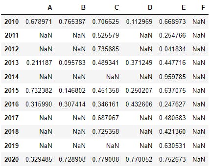
G13). dropna(axis=[0,1], how=[any,all], thresh) Ex-2:
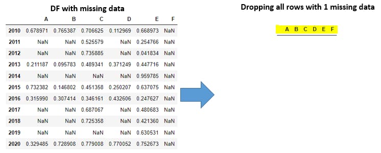
df.dropna()
# by default this function looks like df.dropna(axis=0, how='any')
df.dropna(how='any')
df.dropna(axis=0)
df.dropna(axis=0, how='any')
Explanation: Bydefault with dropna() function we carry axis=0 and how='any'
parameters. axis=0 means row wise, how='any' means in any row if any one value missing then we will drop that perticular row. But in our example all rows are having atleast 1 missing value(if we recall entireF column is missing). So we will get empty dataframe like below.
Output:
G14). dropna(axis=[0,1], how=[any,all], thresh) Ex-3:
df.dropna(axis=1)
# by default this function looks like df.dropna(axis=1, how='any')
df.dropna(axis=1, how='any')
Explanation: Bydefault with dropna() function we carry how='any' parameter alog with axis=1. axis=1 means column wise, how='any' means in any column if any one value missing then we will drop that perticular column. In our example we have only E column which is not having a single missing value and remaining all other columns having atleast 1 missing data.
Output: 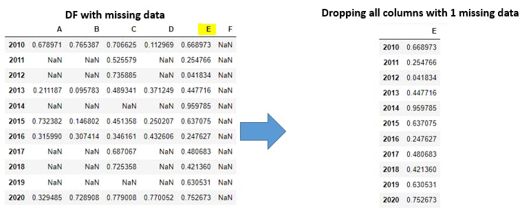
G15). dropna(axis=[0,1], how=[any,all], thresh) Ex-4:
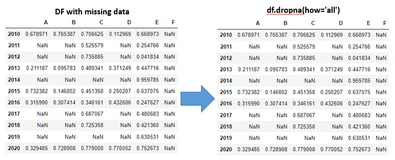
df.dropna(how='all')
#by default this function looks like df.dropna(how='all', axis=0)
df.dropna(how='all', axis=0)
Explanation: how='all' means in given row if all cells are having missing data then that row will get eliminated in the output. axis=0will be added by default to the function. In our example we dont have such rows where all columns data is missing, so we will get our original dataframe as output.
Output:
G16). dropna(axis=[0,1], how=[any,all], thresh) Ex-5:
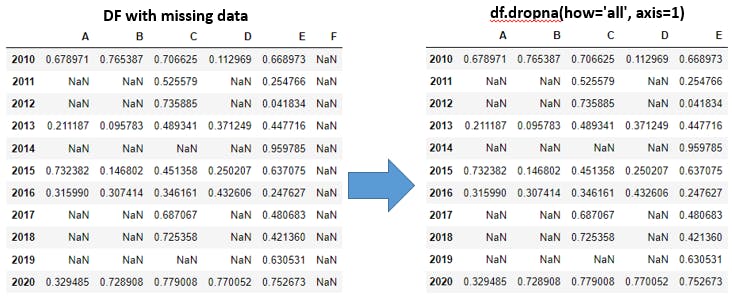
df.dropna(how='all', axis=1)
Explanation: axis=1 means we have to consider columns and how='all' will be considered as in each column if all cells are missing then that column will get eliminated in the output. In our example F column is having all missing data, so it will get eliminated.
Output:
G17). dropna(axis=[0,1], how=[any,all], thresh) Ex-6:
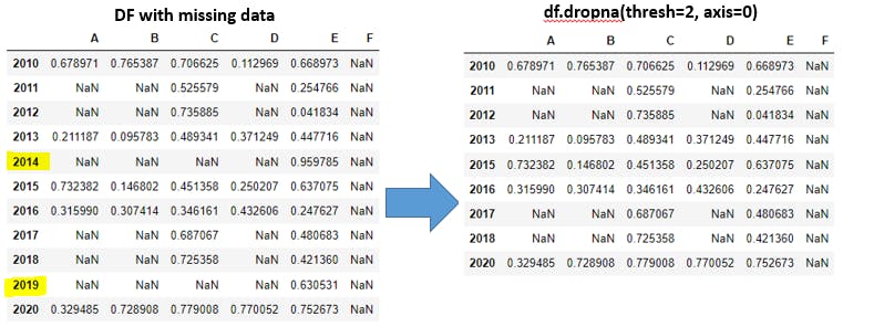
df.dropna(thresh=2, axis=0)
Explanation: axis=0 means row wise, thresh=2 means in each row if we have atleast 2 non-missing data(proper data) then that row will be considered in the output. If any row having lessthan 2 non-missing data then those rows will get eliminated. In 2014, 2019 rows we have only 1 non-missing data so these rows will get eliminated.
Output:
G18). dropna(axis=[0,1], how=[any,all], thresh) Ex-7:
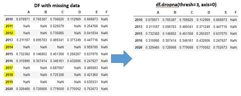
df.dropna(thresh=3, axis=0)
Explanation: axis=0 means row wise, thresh=3 means in each row if we have atleast 3 non-missing data(proper data) then that row will be considered in the output. If any row having lessthan 3 non-missing data then those rows will get eliminated. In 2011, 2012, 2014, 2017, 2018, 2019 rows we have lessthan 3 non-missing data so these rows will get eliminated.
Output:
G19). dropna(axis=[0,1], how=[any,all], thresh) Ex-8:
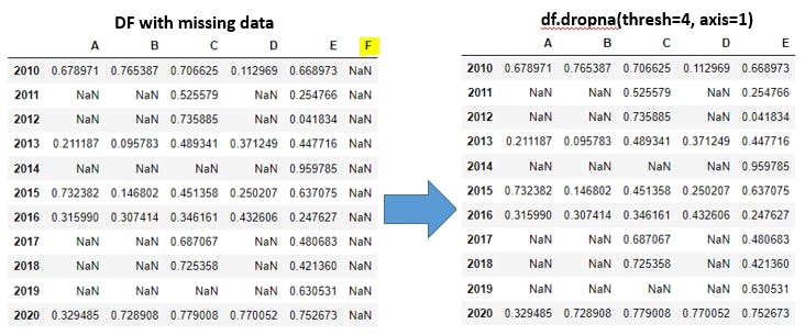
df.dropna(thresh=4, axis=1)
Explanation: axis=1 means column wise, thresh=4 means in each column if we have atleast 4 non-missing data(proper data) then that column will be considered in the output. If any column having lessthan 4 non-missing data then those columns will get eliminated. In Fcolumns all cells are having missing data so it will be eliminated.
Output:
G20). dropna(axis=[0,1], how=[any,all], thresh) Ex-9:
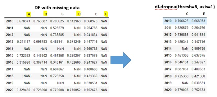
df.dropna(thresh=6, axis=1)
Explanation: axis=1 means column wise, thresh=6 means in each column if we have atleast 6 non-missing data(proper data) then that column will be considered in the output. If any column having lessthan 6 non-missing data then those columns will get eliminated. In A, B, D, Fcolumns lessthan 6 non-missing cells are available so these columns will be eliminated.
Output:
H). Group by in Dataframes:
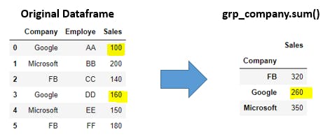
Group by statement is used to group the dataframe columns data into groups and on top of groups we can apply filters or aggregations functions to get the more insights about data.
H1). Sample Data:
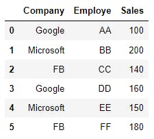
dict1 = {"Company":['Google','Microsoft','FB','Google','Microsoft','FB'],
         "Employe":['AA','BB','CC','DD','EE','FF'],
         "Sales":[100,200,140,160,150,180]}
df = pd.DataFrame(dict1)
df
Explanation: By using python dictionary with 3 keys (Company, Employe, Sales) and each key is having value with list of 6 objects has been used created pandas dataframe.
Output:
H2). Create groups from Dataframe:
grp_company = df.groupby("Company")
grp_company.groups
Explanation: From df dataframe using Company column we are grouping the data with df.groupby("Company") syntax. Finally we are printing the groups with index value from dataframe.
Output:

H3). Checking statistical information:
grp_company.describe()
Explanation: grp_company will contains each group details and describe() function we can get the statistical information about each group.
Output:

H4). Tranpose of statistical matrix:
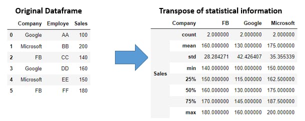
grp_company.describe().transpose()
Explanation: By using transpose() function we flip the matrix such a way that rows become columns and vice versa.
Output:
H5). Aggregation functions:
grp_company.sum()
Explanation: On top of each group we can apply aggregation functions like min(), max(), sum(), avg() to get the more insights of the data.
Output:
I). Combine multiple dataframes:
Pandas offers 3 ways to combine the multiple dataframes so that we can see the data from multiple dataframes as single dataframe with controlling the conditions how to combine. Lets explore one by one.
merge()- If we are aware ofSQLjoins and if we want to perform the SQL like joins then this function will help us. Most of the we will usemerge()function while working in realtime data. This functions comes with more flexibility to control the combining operations.join()- This function is act as a left join inmerge()function. In this we wont specify the what basis join should take place. By default it will join dataframes based on indexes we provide.concat()- This function is little different thatnmerge(), join()functions as it will simply combine the 2 or more dataframes eitherrows wise(vertically)orcolumns wise(horizontally).
I1). Sample Dataframes:
#df1
df1 = pd.DataFrame({'A': ['A0', 'A1', 'A2', 'A3','A4', 'A5'],
                        'B': ['B0', 'B1', 'B2', 'B3', 'B4', 'B999'],
                        'C': ['C0', 'C1', 'C2', 'C3', 'C4', 'C5'],
                        'D': ['D0', 'D1', 'D2', 'D3', 'D4', 'D5']},
                        index=[0, 1, 2, 3, 4, 5])

#df2
df2 = pd.DataFrame({'A': ['A4', 'A5', 'A6', 'A7'],
                        'B': ['B4', 'B5', 'B6', 'B7'],
                        'C': ['C4', 'C5', 'C6', 'C7'],
                        'D': ['D4', 'D5', 'D6', 'D7'],
                        'E': ['E4', 'E5', 'E6', 'E7']},
                         index=[4, 5, 6, 7])

#df3
df3 = pd.DataFrame({'A': ['A7', 'A8', 'A9', 'A10', 'A11'],
                        'B': ['B7', 'B8', 'B9', 'B10', 'B11'],
                        'C': ['C7', 'C8', 'C9', 'C10', 'C11'],
                        'D': ['D7', 'D8', 'D9', 'D10', 'D11']},
                        index=[7, 8, 9, 10, 11])
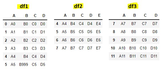
Explanation: We have created 3 dataframes(df1, df2, df3) with index values. These dataframes will be used in below merge() tutorials.
Output:
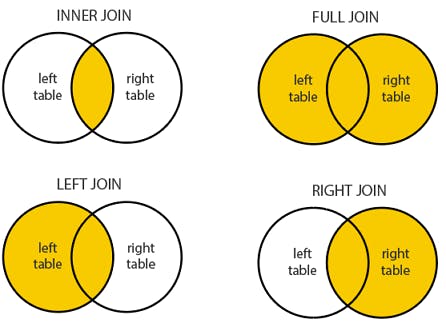
Types of joins we are going to discuss with merge() function as follows:
I2). merge(df1, df2, how='inner') Ex-1: You can skip this example:
df1_inner_df2 = pd.merge(df1, df2, how='inner')
df1_inner_df2

# df1_merge_df2 = pd.merge(df1, df2)
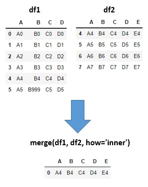
Explanation: In the real world problems we mainly use merge() function over join(), combine() function as with merge() function we can perform SQL like join operations.
In merge() bydefault how=inner and on=indexes will take place. Inner join means all the records which are matching in both dataframes with given columns or indexes will we printed. If we specifically mention about join condition with on= parameter with either columns or indexes inner join will takes place with given columns or indexes else by default join will happend based on indexes given in the dataframe.
Ex:
In this example we have not provided on= parameter, so by default inner join will performed based on indexes of df1, df2. df1 index values =[0, 1, 2, 3, 4, 5] and df2 index values =[4, 5, 6, 7]. out of 2 index lists only [4,5] indexes are matching. Lets explore 4,5 indexes from each dataframe.
df1 index 4=[A4,B4,C4,D4] and df2 index 4=[ A4,B4,C4,D4,E4]. Here we are performing inner join so all matching columns get compared and all are matching.
df1 index 5=[A5,B999,C5,D5] and df2 index 4=[ A5,B5,C5,D5,E5]. Here column B is having different values(B999 != B5) so index B will not get printed.
Output:
I3). merge(df1, df2, how='inner') Ex-2:
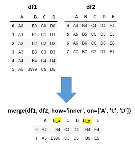
df1_inner_df2 = pd.merge(df1, df2, how='inner', on=['A', 'C', 'D'])
df1_inner_df2

# SQL Query for above python code:
SELECT df1.*, df2.*
FROM df1
INNER JOIN df2
ON (df1.A=df2.A AND df1.C=df2.C AND df1.D=df2.D)
Explanation: Here also we are doing inner join with how='inner' parameter but additionally we are giving on=['A', 'C', 'D'] parameter to perform inner join based on A, C, D columns. In both df1, df2 dataframes if any row having same A, C, D column values then those rows will get printed.
Ex:
In 4,5 indexes from both dataframes A, C, D columns are matching so 4,5 indexes will get printed. If we observe column names we have B_x, B-y columns. Here B_x is coming from df1 and B_y is coming from df2. Just to get the clear output pandas will automatically append these _x, _ycharacters to matching columns in both dataframe if they have different data.
Output:
I4). merge(df1, df2, how='left', on=['A', 'D']):
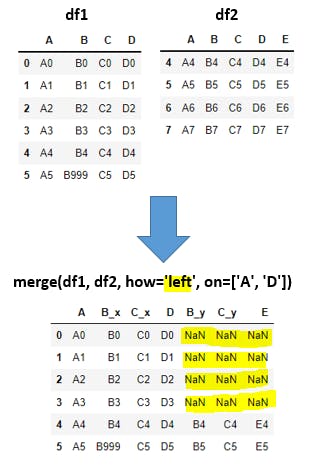
df1_left_df2 = pd.merge(df1, df2, how='left', on=['A', 'D'])
df1_left_df2

# SQL Query for above python code:
SELECT df1.*, df2.*
FROM df1
LEFT JOIN df2
ON (df1.A=df2.A AND df1.D=df2.D)
Explanation: We are performing left join between df1, df2 with A,Dcolumns as join condition. Left Join means all the rows from left table(df1) and matching row values from right table(df2) will have proper values. Non-matching rows from right table(df2) will have NaN i.e. Not a Number. Just to avoid the ambiguity between df1, df2 column names _x for df1column names, _y for df2 column names will be appened.
Note: Column names A, D will remain same because these columns are matching between 2 dataframes and column nameE will also remain same because column E is not ambiguous. In output all rows[6] from left df, matching rows[2] from right df will come. Total rows=6.
Output:
I5). merge(df1, df2, how='right', on=['A', 'D']):
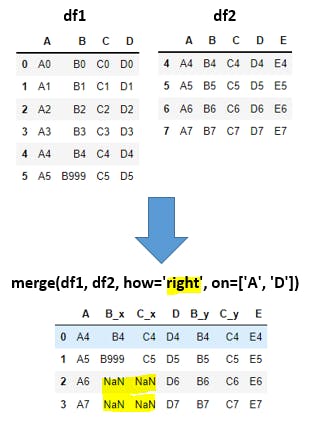
df1_right_df2 = pd.merge(df1, df2, how='right', on=['A', 'D'])
df1_right_df2

# SQL Query for above python code:
SELECT df1.*, df2.*
FROM df1
RIGHT JOIN df2
ON (df1.A=df2.A AND df1.D=df2.D)
Explanation: We are performing right join between df1, df2 with A,Dcolumns as join condition. Right Join means all the rows from right table(df2) and matching row values from left table(df1) will have proper values. Non-matching rows from left table(df1) will have NaN i.e. Not a Number. Just to avoid the ambiguity between df1, df2 column names _x for df1 column names, _y for df2 column names will be appened. In output all rows[4] from right df, matching rows[2] from left df will come. Total rows=4.
Output:
I6). merge(df1, df2, how='outer', on=['A', 'D']):
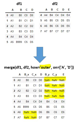
df1_outer_df2 = pd.merge(df1, df2, how='outer', on=['A', 'D'])
df1_outer_df2

# SQL Query for above python code:
SELECT df1.*, df2.*
FROM df1
FULL OUTER JOIN df2
ON (df1.A=df2.A AND df1.D=df2.D)
Explanation: We are performing outer join between df1, df2 with A,Dcolumns as join condition. OuterJoin means all rows from left table(df1) and all rows from right table(df2) will be displayed but non-matching rows from both the tables will be displayed as NaN i.e. Not a Number. In output (leftDF[6]-matching[2]) + (matching[2]) + (rightDF[4]-matching[2]) = 4+2+2 =8 total rows will be displayed.
Output:
I7). join() function:
# df1 declaration
df1 = pd.DataFrame({'A': ['A0', 'A1', 'A2'],
                     'B': ['B0', 'B1', 'B2']},
                      index=['K0', 'K1', 'K2'])

# df2 declaration
df2 = pd.DataFrame({'C': ['C0', 'C2', 'C3'],
                    'D': ['D0', 'D2', 'D3']},
                      index=['K0', 'K2', 'K3'])

#Join statement
df1_join_df2 = df1.join(df2)
df1_join_df2
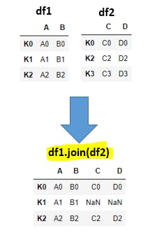
Explanation: By default join() function acts as left join in the SQL side. Here we wont specify on what bases it should join, it will consider indexes for joining. In real world applications merge() function used very frequently. In output all rows from left table(df1) and matching rows from right table(df2) will have proper values and non-matching rows from right table(df2) will have NaN.
Output:
I8). concat([df1, df2, df3]):
Lets use the old dataframes in this example as below.
#df1
df1 = pd.DataFrame({'A': ['A0', 'A1', 'A2', 'A3','A4', 'A5'],
                        'B': ['B0', 'B1', 'B2', 'B3', 'B4', 'B999'],
                        'C': ['C0', 'C1', 'C2', 'C3', 'C4', 'C5'],
                        'D': ['D0', 'D1', 'D2', 'D3', 'D4', 'D5']},
                        index=[0, 1, 2, 3, 4, 5])

#df2
df2 = pd.DataFrame({'A': ['A4', 'A5', 'A6', 'A7'],
                        'B': ['B4', 'B5', 'B6', 'B7'],
                        'C': ['C4', 'C5', 'C6', 'C7'],
                        'D': ['D4', 'D5', 'D6', 'D7'],
                        'E': ['E4', 'E5', 'E6', 'E7']},
                         index=[4, 5, 6, 7])

#df3
df3 = pd.DataFrame({'A': ['A7', 'A8', 'A9', 'A10', 'A11'],
                        'B': ['B7', 'B8', 'B9', 'B10', 'B11'],
                        'C': ['C7', 'C8', 'C9', 'C10', 'C11'],
                        'D': ['D7', 'D8', 'D9', 'D10', 'D11']},
                        index=[7, 8, 9, 10, 11])
df1_df2_df3_ver_concat = pd.concat([df1, df2, df3])
df1_df2_df3_ver_concat

# df1_df2_df3_ver_concat = pd.concat([df1, df2, df3], axis=0)
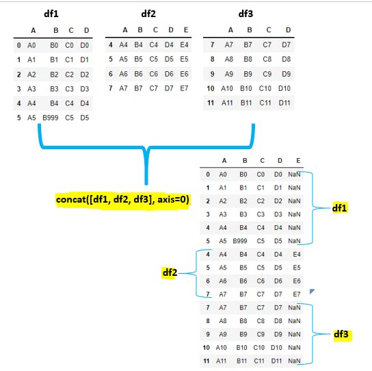
Explanation: concat() function will be used with axis=[0,1] parameter. If we give axis=0 then all given dataframes(df1, df2, df3) will be combined vertical manner like below. By default concat() function will have axis=0 parameter. In the output all non-existing rows will be replaced with NaN while combining.
Output:
I). concat([df1, df2, df3] axis=0):
df1_df2_df3_hor_concat = pd.concat([df1, df2, df3], axis=1)
df1_df2_df3_hor_concat
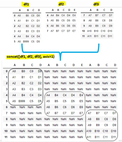
Explanation: concat() function will be used with axis=[0,1] parameter. If we give axis=1 then all given dataframes(df1, df2, df3) will be combined horizontal manner like below. In the output all non-existing rows will be replaced with NaN while combining.
Output:
Conclusion:
I hope you have learned Pandas concepts with simple examples.
Happy Learning...!!

