NumPy - Python for Data Science

Table of Content:

In this Numpy tutorial, we will be learning below concepts.

• Prerequisites:
• A). Introduction to Numpy:
• B). Importing Package:
• C). Creating Numpy Array in different ways:
• D). Shape, ReShape of Numpy Array:
• E). Indexing and Slicing of Numpy Array:
• F). Numpy special Arrays:
• G). Copying or Duplicating Numpy Arrays:
• H). Broadcasting in Numpy:
• I). Numerical operations on Numpy Array:
• J). Matrices vs Numpy Ndarray:
• K). Numpy inbuilt functions:
• Conclusion:

---

Prerequisites:

Numpy concepts are to apply numerical operations on top of Python Data structures. With the help of Numpy we can easily able to get the required numerical calculations in real time Data Analysis and Data science fields.
Ex: If we understand anything in between from basics of mathematical operations till advanced calculus, we can apply Numpy concepts to get things done in our analysis.

---

A). Introduction:

• Numpy stands for Numerical Python.
• Numpy is a python fundamental package for scientific computing. Which is used to create or manipulate the multidimensional arrays or matrices. To perform complex mathematical operations, statistical computation, trigonometric operations and solving algebra problems.
• Numpy arrays are mush faster than Python lists while computing and at runtime. While a Python list can contain different data types within a single list, all of the elements in a NumPy array should be homogeneous.
  

---

B). Import package:

import numpy as np

Explanation: import key word is used to import the required package into our code. as keyword is used for giving alias name for given package. numpy is the numerical python package used to create numerical arrays in this tutorial. Example: numpy is the package and npis the alias name or short name for numpy.

---

C). Creating Numpy Array:

We have multiple ways to create numpy arrays. In this section we will see how to create numpy arrays with below methods.

• np.arange() : When we know staring, ending numbers with step size but not sure on how many number of values will come.
• np.linspace() : When we know starting, ending numbers with number of values in between but not sure on step size.
• np.array() : With given any python object(List, Tuple) or any one of the above.

C1). np.arange() function :

• np.arange() function will be useful when we know the starting point, ending point and step size(difference between each element to its next element in the array). Case: If we need elements between 40, 90 values with step size=2. We will see few of the examples how we can utilize this function.

C1 - Ex1). np.arange() function with End value:

a = np.arange(10)
a

Explanation: Only ending point given. Ifnp.arange() function is having one parameter then by default it will be considered as end value and from zero to given number with step size =1 will be printed in the output array.
Ex: Here we have 10 as a parameter. In this case starting point = 0, ending point = 10 and step size =1. In the output we will be having list of values from 0 to 10 with space of 1 i.e. 0, 1, 2, 3, 4, 5, 6, 7, 8, 9. Here ending point is excluded in the output.
Output:

C1 - Ex2). np.arange() function with End value:

a = np.arange(10)
type(a)

Explanation: By using type() method we can cross check that output array is a numpy - ndarray i.e. Numpy- N Dimensional array.
Output:

C1 - Ex3). np.arange() function with Start, End values:

a = np.arange(0, 10)
a

Explanation: Starting, Ending points given. Ifnp.arange() function is having two parameters then first parameter is starting point and second parameter is ending point with step size = 1 will be printed in the output array.
Ex: Here we have starting point = 0, ending point = 10 and step size =1. In the output we will be having list of values from 0 to 10 with space of 1 i.e. 0, 1, 2, 3, 4, 5, 6, 7, 8, 9. Here ending point is excluded in the output.
Output:

C1 - Ex4). np.arange() function with Start, End, Step values:

a = np.arange(0, 10, 2)
a

Explanation: Starting, Ending, Step size given. Output array will contain from starting point, till ending point with step size value.
Ex: Here start=0, End=10 and Step=2 has given. In the output array first value will be 0, second value will be 0 + 2 i.e 2, third value will be 2 + 2 i.e. 4, forth value will be 4 + 2 i.e. 6 and firth value will be 6 + 2 i.e. 8. Here output will stop because ending point will be excluded by default so for next iteration we wont get any value in output.
Output:

C1 - Ex5). np.arange() function with Start, End, Step, Datatype values:

a = np.arange(0, 10, 2, float)
a

Explanation: Starting, Ending, Step size, datatype given. Output array will contain from starting point, till ending point with step size value. All values will be floating point numbers in the output.
Ex: Here start=0, End=10 and Step=2 has given. In the output array first value will be 0., second value will be 0 + 2 i.e 2.0, third value will be 2 + 2 i.e. 4.0, forth value will be 4 + 2 i.e. 6.0 and firth value will be 6 + 2 i.e. 8.0. Here output will stop because ending point will be excluded by default so for next iteration we wont get any value in output.

Output:

C1 - Ex6). np.arange() function with Start, End, Step values for floating numbers:

a = np.arange(0.25, 10.25, 2)
a

Explanation: Here we are applying np.arange() function on floating numbers. Output will be having floating numbers by default.
Ex: Here start=0.25, End=10.25 and Step=2 has given. In the output array first value will be 0.25, second value will be 0.25 + 2 i.e 2.25, third value will be 2.25 + 2 i.e. 4.25, forth value will be 4.25 + 2 i.e. 6.25 and firth value will be 6.25 + 2 i.e. 8.25. Here output will stop because ending point will be excluded by default so for next iteration we wont get any value in output.

Output:

C2). np.linspace() function :

• np.linspace() function will be useful when we know starting point, ending point and number of values in between but not sure on step size of each element to its next element. Case: If we need 20 elements (which are equally spaced one to its next element) between 40, 90 values. We will see few of the examples how we can utilize this function.

C2 - Ex1). np.linspace() function with Start, End, default no..of element values:

a = np.linspace(1,10)  #default number of elements=50
a

Explanation: Here we have given only starting, ending points but not number of values we want. In this case by default it will be 50. We are creating a numpy array with values between 1, 10 and number of elements =50.
Output:

C2 - Ex2). np.linspace() function with Start, End, default no..of element values:

a = np.linspace(1,10)  #default number of values=50
print(a)
print("Type of array: ", type(a))
print("Length of array: ", len(a))

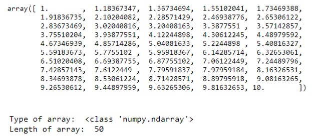
Explanation: Here we have given only starting, ending points but not number of values we want. In this case by default it will be 50. We are creating a numpy array with values between 1, 10 and number of elements =50.
Using type() function we can observe that output array is Numpy- N Dimesional array.
Using len() function we can see that array contains 50 elements.
Output:

C2 - Ex3). np.linspace() function with Start, End, No..of Elements values:

a = np.linspace(0,35,6) 
print(a)
print("Type of array: ", type(a))
print("Length of array: ", len(a))

Explanation: Here we have given only starting, ending points and number of values we want. In this case from 0 to 35 if we obtain 6 values between then we will get below output.
Using type() function we can observe that output array is Numpy- N Dimesional array.
Using len() function we can see that array contains 6 elements. This example we can easily relate that values are multiples of number 7 from 0 i.e. [0, 7, 14, 21, 35].
Output:

C3). np.array() function :

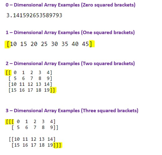
• np.array() function is most used approach to create numpy arrays. With given any one of python list, tuple we use this function to create numpy arrays. Before looking into this function, lets understand the different dimensionalities of Numpy arrays. Based on square brackets we can easily identify the dimensions of array. For 1-D Array will have 1 square bracket at starting, ending positions. For 2-D array 2 square brackets, for 3-D array 3 square brackets and so on.
  

Ex:

C3 - Ex1). np.array() function with constant value : 0-Dimensional array:

a = np.array(40)

print("array : ", a)
print("Type of a:", type(a))
print("Dimentions of a: ", np.ndim(a))
print("Datatype of a: ", a.dtype)

Explanation: This example shows how to create numpy array with one scalar value i.e. 40 has given as a parameter to np.array() function. This is an example for 0-Dimensional array.

• First line in the output shows the array value. We have 40 as a array value.
• Second line is the type of array with type() function, here it is N-Dimesional array.
• In third line with the help of np.ndim() function we can see the dimensionality of the numpy array, here given array is 0-Dimensional array.
• Fourth line is for checking datatype of array values it contains, here we know that 40 is the Integer type.

Output:

C3 - Ex2). np.array() function with List : 1-Dimensional array:

a = np.array([0,2,4,6,8,10,12])

print("Array : ", a)
print("Type of a:", type(a))
print("Dimentions of a: ", np.ndim(a))
print("Datatype of a: ", a.dtype)

Explanation: This example shows how to create numpy array with list of values i.e. [0,2,4,6,8,10,12] has given as a parameter to np.array() function. This is an example for 1-Dimensional array.

• First line in the output shows the array value. We have [0,2,4,6,8,10,12] as a array values.
  
• Second line is the type of array with type() function, here it is N-Dimesional array.
  
• In third line with the help of np.ndim() function we can see the dimensionality of the numpy array, here given array is 1-Dimensional array.
  
• Fourth line is for checking datatype of array values it contains, here we know that 0,2,4,6,8,10,12 given values are Integer type.

Output:

C3 - Ex3). np.array() function with Numpy Array : 1-Dimensional array:

a = np.array(np.arange(10,50,5))

print("Array : ", a)
print("Type of a:", type(a))
print("Dimentions of a: ", np.ndim(a))
print("Datatype of a: ", a.dtype)

Explanation: This example shows how to create numpy array with output of np.arange() function i.e. [10 15 20 25 30 35 40 45] has given as a parameter to np.array() function. This is an example for 1-Dimensional array.

• First line in the output shows the array value. We have [10 15 20 25 30 35 40 45] as a array values.
  
• Second line is the type of array with type() function, here it is N-Dimesional array.
  
• In third line with the help of np.ndim() function we can see the dimensionality of the numpy array, here given array is 1-Dimensional array.
  
• Fourth line is for checking datatype of array values it contains, here we know that 10 15 20 25 30 35 40 45 given values are Integer type.

Output:

C3 - Ex4). np.array() function with 2D matrix: 2-Dimensional array:

a = np.array([[1,2,3],[4,5,6]])

print("Array : \n", a)
print("Type of a:", type(a))
print("Dimentions of a: ", np.ndim(a))
print("Datatype of a: ", a.dtype)

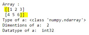
Explanation: This example shows how to create numpy array with 2-D matrix given to np.array() function. If we observe starting and ending 2 square brackets are there.

• First line in the output shows the array value.
  
• Second line is the type of array with type() function, here it is N-Dimesional array.
  
• In third line with the help of np.ndim() function we can see the dimensionality of the numpy array, here given array is 2-Dimensional array.
  
• Fourth line is for checking datatype of array values it contains, here we know that given values are Integer type.

Output:

C3 - Ex5). np.array() function with 3D matrix 3-Dimensional array:

a = np.array([[[ 0,  1,  2],[ 3,  4,  5]], [[ 6,  7,  8],[ 9, 10, 11]]])

print("Array : \n", a)
print("\nType of a:", type(a))
print("Dimentions of a: ", np.ndim(a))
print("Datatype of a: ", a.dtype)

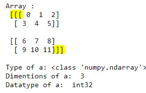
Explanation: This example shows how to create numpy array with 3-D matrix given to np.array() function. If we observe starting and ending 3 square brackets are there.

• First line in the output shows the array value.
  
• Second line is the type of array with type() function, here it is N-Dimesional array.
  
• In third line with the help of np.ndim() function we can see the dimensionality of the numpy array, here given array is 3-Dimensional array.
  
• Fourth line is for checking datatype of array values it contains, here we know that given values are Integer type.

Output:

---

D). Shape, ReShape of Numpy Array:

Identifying the shape of numpy array and converting given array shape into required shape we want for our analysis will be easliy done by below functions in Numpy package.

• shape() : Used to get shape(no..of Rows, no..of Columns) of Numpy array.
• reshape() : Used to change the dimensions and shape of Numpy array.

D1). shape() function with constant value: 0-Dimensional array:

a = np.array(45)

print("Array: ", a)
print("Dimensions: ", np.ndim(a))
print("Shape: ", np.shape(a))  # Approach-1

a = np.array(45)

print("Array: ", a)
print("Dimensions: ", np.ndim(a))
print("Shape: ", a.shape)  # Approach-2

Explanation: With np.array() function we have created 0-Dimensional array with 45 constant value. With np.dim() function we can get the dimentionality of an array. We can use any one of np.shape(a) or a.shape methods to print the shape (no..of Rows, no..of Columns) of an array. Just to avoid ambiguity going forward we will be using np.shape() function.
Ex: In the below example we have created array with constant value, we know that this is 0-Dimentional array. For 0-D array np.shape() function will give blank values as below.
Output:

D2). shape() function with List: 1-Dimensional array:

a = np.array([1,2,3,4,5,6,7,8,9,10])

print("Array:", a)
print("Dimensions: ", np.ndim(a))
print("Shape: ", np.shape(a))

Explanation: With np.array() function we have created 1-Dimensional array with Python List . With np.dim() function we can get the dimentionality of an array i.e. 1-D array. With np.shape(a) function we can get the shape (no..of Rows, no..of Columns) of an array. Here 1-D array will be having only no..of rows without any columns. Here we have 10 rows. Note: Please dont get confuse with rows and columns here. Bydefault any 1-D array will be treated in vertical manner. With 2-D array examples we will understand np.shape() function clearly.
Output:

D3). shape() function with 2D Matrix: 2-Dimensional array:

a = np.array([[0, 1, 2, 3, 4], [5, 6, 7, 8, 9]])

print("Array:\n", a)
print("\nDimensions: ", np.ndim(a))
print("Shape: ", np.shape(a))

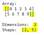
Explanation: We have created 2D numpy array with 2D matrix. The np.ndim() function will give 2 as a dimentionality of an array. If we observe in the shape of array it is having 2 rows and 5 columns and printed as (2, 5).
Output:

D4). shape() function with 3D Matrix: 3-Dimensional array:

a = np.array([[[ 0,  1,  2,  3],[ 4,  5,  6,  7],[ 8,  9, 10, 11]],
             [[12, 13, 14, 15],[16, 17, 18, 19],[20, 21, 22, 23]]])

print("Array:\n", a)
print("\nDimensions: ", np.ndim(a))
print("\nShape: ", np.shape(a))

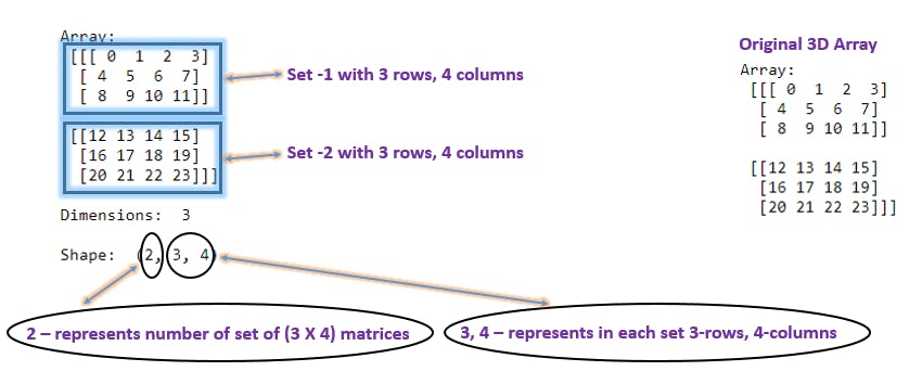
Explanation: With given 3D matrix we have created 3D array. With np.ndim() we can see it is 3D array. np.shape() functions returns (2, 3, 4). 2 means 2 set of (3, 4) matrices there. 3, 4 means in each set we have 3-rows, 4-columns. If below diagram we can easily digest the 3D Array shape.
Output:

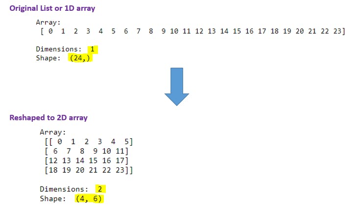
D5). reshape() function - 1D to 2D Array:

li = np.arange(24)
a = li.reshape(4, 6)

print("Array:\n", a)
print("\nDimensions: ", np.ndim(a))
print("Shape: ", np.shape(a))

a = np.arange(24).reshape(4, 6)

Explanation: We have a list or 1D array with 24 values. With reshape() function we have converted the 1D array into 2D array. In reshape function we have to give dimensions and multiplication of these dimensions should be equal to number of values in the original array. Here 4 X 6 = 24.
We can do this in 2 lines of the code as first code or in single line we can do like second code snippet. Going forward we will be using single code snippet for reshaping the original array.
Output:

D6). reshape() function - 1D to 3D Array:

a = np.arange(24).reshape(2, 3, 4)

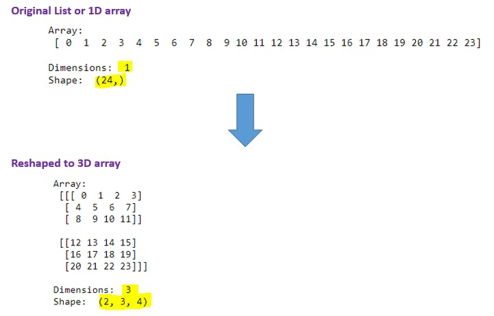
Explanation: Here it must be 2 X 3 X 4 = 24. Here we are converting 1D to 3D array using reshape() function. We have seen 3D array explanation in previous section.
Output:

D7). reshape() function - 2D to 3D Array:

a = (np.arange(24).reshape(4, 6)).reshape(2, 3, 4)

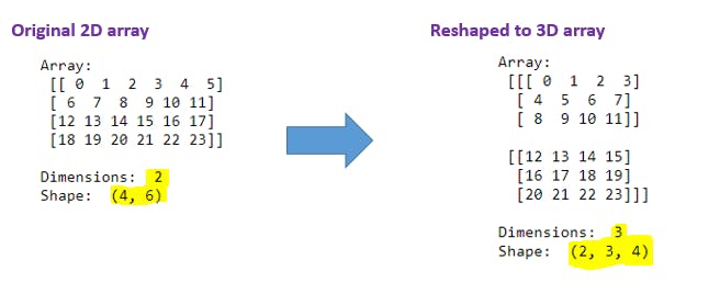
Explanation: With (np.arange(24).reshape(4, 6)) code we have 2D array in our hand and then outer side we have applied reshape(2, 3, 4) to convert 2D array to 3D array. Note that while converting into different dimensions multiplication of shape must be equal to its original array element count like 24 = 4 X 6 = 2 X 3 X 4.
Output:

D8). reshape() function - 3D to 2D Array:

a = (np.arange(24).reshape(2,3,4)).reshape(4,6)

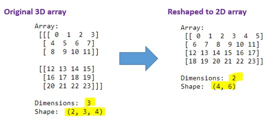
Explanation: With (np.arange(24).reshape(2,3,4)) code we have 3D array in our hand and then outer side we have applied reshape(4,6) to convert 3D array to 2D array. Note that while converting into different dimensions multiplication of shape must be equal to its original array element count like 24 = 4 X 6 = 2 X 3 X 4. We can convert any dimensional array into required dimensional array if and only if given multiplication matches.
Output:

---

E). Indexing and Slicing of Numpy Array :

• Indexing: By using index we can access the elements in a Numpy array just like accessing elements in List, Tuple.
• Slicing : If we want select an element or 1 portion(list of elements in array) of Numpy array we use this concept. A[start:stop:step] this concept applicable to slicing the Numpy array aswell.
• Boolean Indexing: By using any comparison operators(<, <=, >, >=, ==) on top of numpy array will generate the boolean indexing array.

E1). Indexing and slicing 1D array : Array[ :: ]

a = np.array([0, 1, 2, 3, 4, 5, 6, 7, 8, 9])

print("Array:", a)
print("Array Length:", len(a))

print("\n*********** :Indexing Examples: ***********")
print("1.Access first elements in Array: ", a[0])
print("2.Access last elements in Array with [-1] index: ", a[-1])
print("3.Access last elements in Array : ", a[9])
print("4.Access 3rd elements in Array: ", a[2])

print("\n*********** :Slicing Examples: ***********")
print("1.Slice the array from 4th element to end: ", a[3:])
print("2.Slice the such that only even indexes should come: ", a[::2])
print("3.Slice the such that only odd indexes should come: ", a[1::2])
print("4.Print the array in reverse order: ", a[::-1])

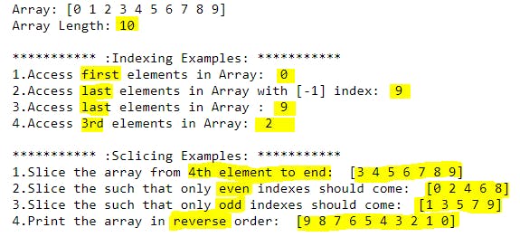
Explanation: For 1D array we can use a[start, end, step].
Indexing : For Numpy arrays index will start with 0. For accessing first element we have use a[0] which means a is the numpy array name and 0 is the index. Similarly for accessing last element we have 2 options. We can use length -1 i.e. a[9] to get the last element or we can use -1 like a[-1]. Like this if we want to access n th element in array, we have to pass n-1 as a index value to array.

Slicing : If we want to get small portion of array we have use [Start:Stop:Step] approach. To get subarray from 4th element to end we can use a[3:]. Here we are saying print from index 3 to end. To print even indexed elements we can use a[::2]. It means print elements from start to end with step size 2. Similarly for odd index positions we will use a[1::2]because we know that first odd number is 1 till end with step size 2. To reverse the given numpy array in simply way is use the -1 as step size like a[::-1]. Here we are expecting ouput from start to end with reverse order.
Output:

E2). Indexing and slicing 2D array : Array[ :: , :: ]

a = np.arange(24).reshape(4, 6)

print("Array:\n", a)
print("\nArray Length:", np.size(a))

print("\n*********** :Indexing Examples: ***********")
print("1.Print 16 value:", a[2, 4])
print("2.Print 21 value:", a[3, 3])
print("3.Print 9 value:", a[1, 3])
print("4.Print 23 value:", a[-1, -1])

print("\n*********** :Slicing Examples: ***********")
print("1.Access 1st row in Array: ",  a[0,:])
print("2.Access last row in Array: ", a[-1,:])
print("3.Access first column in Array: ", a[:,0])
print("4.Access last column in Array: ",  a[:,-1])

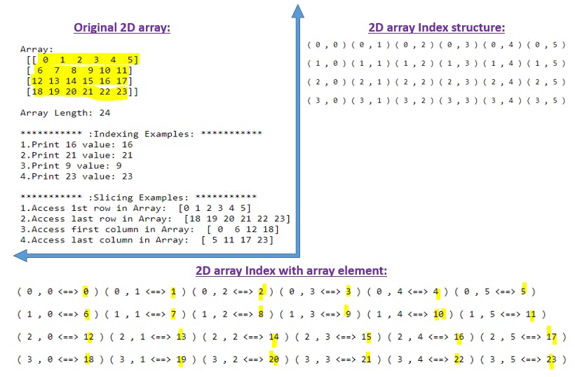
Explanation: For 2D array we use [ :: , :: ] format which is separated with , and left side we can do indexing or slicing for rows, right side we can do indexing or slicing for columns because it is 2D array we must deal with rows and columns. In each side we can apply list indexing operations like [start:end:step].
Indexing Examples : If we see the below screenshot in row index=2 and column index=4 we get the value=16. Similar way by seeing below heading 2D array Index with array element: we have indexes by row, column wise to get the perticular array value.
Slicing Examples : To get entire first row we use a[ 0 , : ]syntax. Which means at row indexing we are expecting to print first row and with column indexing we are expecting all columns from first row.

Output:

E3). Indexing and slicing 3D array : Array[ :: , :: , :: ]

a = np.arange(24).reshape(2, 3, 4)

print("Array:\n", a)
print("\nArray Length:", np.size(a))

print("\n*********** :Indexing Examples: ***********")
print("1.Print 5 value:", a[0, 1, 1])
print("2.Print 8 value:", a[0, 2, 0])
print("3.Print 17 value:", a[1, 1, 1])
print("4.Print 23 value:", a[1, 2, 3])

print("\n*********** :Slicing Examples: ***********")
print("1.Access 1st set in 3D Array: \n",  a[0 , : , : ])
print("2.Access 2nd set in 3D Array: \n",  a[1 , : , : ])
print("3.Access 1st column in all set in 3D Array: \n",  a[: , : , 0 ])
print("4.Access 1st row in all set in 3D Array: \n",  a[: , 0 , : ])

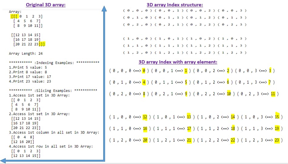
Explanation: For 3D array we use [ :: , :: , :: ] format which is separated with , and 1st one is used for set selection and 2nd one used for indexing or slicing for rows, and 3rd one used for indexing or slicing for columns because it is 3D array we must deal with Sets , rows and columns. In each side we can apply list indexing operations like [start:end:step].
Indexing Examples : If we see the below screenshot to index any value we have to use set value, row value, column value. To get value 5 it is available in set value =0, row value=1 and column value =1 .
Slicing Examples : To get entire first row we use a[ :, 0 , : ]syntax. Which means select values in all sets, in each set select only row=1 and all columns.

Output:

E4). Boolean Indexing of Numpy Array:

# Given 2D numpy array.
a = np.array(np.arange(40,60).reshape(4,5))
print("Array:\n",a)

# Check each value odd or even number in given numpy array 
print("Check each value in numpy array is even or odd number:\n")
print(a%2==0)

print("\nConvert Boolean values into Integers(0,1):")
b = a%2==0
print(b.astype(int))

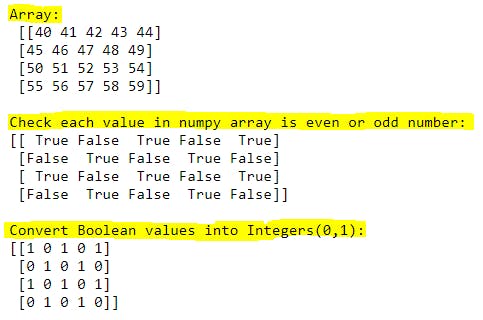
Explanation: By using any comparison operators(<, <=, >, >=, ==) on top of numpy array will generate the boolean indexing array. With np.arange(40,60).reshape(4,5) we are crating 2D numpy array. Array will be having 4 X 5 = 20 elements in it. With a%2==0 code, we are checking each element even or odd value. Finally this code will generate 4 X 5 size boolean array having true or false values in it. We can convert boolean values(true, false) into integer values(0,1) by using type conversion calledastype(int) function.
Output:

---

F). Numpy special Arrays:

In this section we will be learning about ones(), ones_like(), zeros(), zeros_like(), empty(), full(),transpose() special functions of numpy arrays.

• np.ones() : To create numpy array with data as 1 for given dimensions.
• np.ones_like() : To create numpy array with data as 1 with same size as given numpy array.
• np.zeros() : To create numpy array with data as 0 for given dimensions.
• np.zeros_like() : To create numpy array with data as 0 with same size as given numpy array.
• np.empty() : To create an empty numpy array for given shape.
• np.full() : To create numpy array with given data and given shape or dimension.
• np.transpose() : To change the rows into columns and columns into rows for numpy array.
• np.identity() : To create n X n identity square matrix where all diagonal elements set to 1 and rest of the elements set to 0.
• np.eye() : Works just like np.identity() function but it also creates n X m rectangle identity matrix where we mention the position of diagonal elements having 1 and rest all elements to 0.

F1). ones() function:

print("***** Ones() Example: with float type. *****")
a = np.ones(5)
print("Array:\n",a)
print("Array Dimension:", a.ndim)

print("\n***** Ones() Example: with integer type. *****")
a = np.ones(5, dtype='int')
print("Array:\n",a)
print("Array Dimension:", a.ndim)

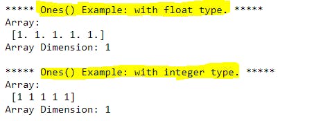
Explanation: ones() function will be useful when we want to create a numpy array with all elements set to 1 or 1. based on datatype with given dimensions. Bydefault all values will be floating points like (1.), we can change the datatype of each value using dtype=int parameter to integer values like (1). With a.ndim argument we can able to see the dimensions of the array.
Ex: In ones() function we are giving 5 which means 1D array having 5 elements and dtype='int' which means output should be in integer datatype.
Output:

F2). ones() function for 2D, 3D arrays:

print("***** Ones() Example 2D Array *****")
a = np.ones((2,3), dtype='int')
print("Array:\n",a)
print("Array Dimension:", a.ndim)

print("\n***** Ones() Example 3D Array *****")
a = np.ones((2,3,4), dtype='int')
print("Array:\n",a)
print("Array Dimension:", a.ndim)

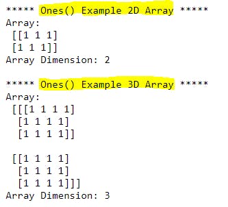
Explanation: We can apply these special functions for higher dimensional arrays aswell. We will be giving the required dimensions like (2,3) or (2,3,4). We can cross check the dimensions with ndim argument.
Output:

F3). ones_like() function for 1D,2D,3D arrays:

print("********** ones_like() Example 1D Array **********")
given_array = np.array([8,4,5,6,3])
target_array = np.ones_like(given_array)
print("Given Array:\n",given_array)
print("\nTarget Array:\n",target_array)
print("\nGiven_array Dimension:", given_array.ndim)
print("Target_array Dimension:", target_array.ndim)

print("\n********** ones_like() Example 2D Array **********")
given_array = np.arange(6).reshape(2,3)
target_array = np.ones_like(given_array)
print("Given Array:\n",given_array)
print("\nTarget Array:\n",target_array)
print("\nGiven_array Dimension:", given_array.ndim)
print("Target_array Dimension:", target_array.ndim)

print("\n********** ones_like() Example 3D Array **********")
given_array = np.arange(24).reshape(2,3,4)
target_array = np.ones_like(given_array)
print("Given Array:\n",given_array)
print("\nTarget Array:\n",target_array)
print("\nGiven_array Dimension:", given_array.ndim)
print("Target_array Dimension:", target_array.ndim)

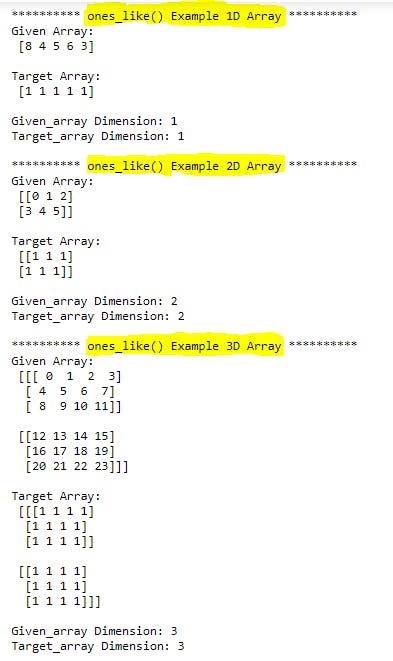
Explanation: ones(), ones_like() functions serve the same functionality. By using ones_like() function also we can able to create a numpy array with all elements =1 but for dimensions purpose, we will be giving reference numpy array. If we give 2D array array as a reference, 2D array with all elements will be 1.
Ex: In below examples we have 1D, 2D, 3D numpy arrays along with their ones_like arrays with same dimensions.
Output:

F4). zeros() function for 1D, 2D, 3D arrays:

print("***** Zeros() Example 1D Array *****")
a = np.zeros(5, dtype='int')
print("Array:\n",a)
print("Array Dimension:", a.ndim)

print("\n***** Zeros() Example 2D Array *****")
a = np.zeros((2,3), dtype='int')
print("Array:\n",a)
print("Array Dimension:", a.ndim)

print("\n***** Zeros() Example 3D Array *****")
a = np.zeros((2,3,4), dtype='int')
print("Array:\n",a)
print("Array Dimension:", a.ndim)

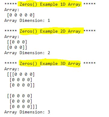
Explanation: Just like ones() function, we can use zeros() function to create a numpy array with given dimensions by setting all elements to 0. We can use zeros() function for any given dimension.
Output:

F5). zeros_like() function for 1D,2D,3D arrays:

print("********** zeros_like() Example 1D Array **********")
given_array = np.array([8,4,5,6,3])
target_array = np.zeros_like(given_array)
print("Given Array:\n",given_array)
print("\nTarget Array:\n",target_array)
print("\nGiven_array Dimension:", given_array.ndim)
print("Target_array Dimension:", target_array.ndim)

print("\n********** zeros_like() Example 2D Array **********")
given_array = np.arange(6).reshape(2,3)
target_array = np.zeros_like(given_array)
print("Given Array:\n",given_array)
print("\nTarget Array:\n",target_array)
print("\nGiven_array Dimension:", given_array.ndim)
print("Target_array Dimension:", target_array.ndim)

print("\n********** zeros_like() Example 3D Array **********")
given_array = np.arange(24).reshape(2,3,4)
target_array = np.zeros_like(given_array)
print("Given Array:\n",given_array)
print("\nTarget Array:\n",target_array)
print("\nGiven_array Dimension:", given_array.ndim)
print("Target_array Dimension:", target_array.ndim)

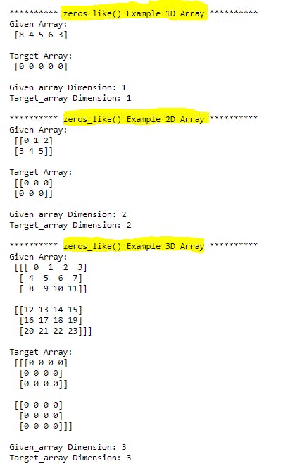
Explanation: zeros(), zeros_like() functions serve the same functionality. By using zeros_like() function also we can able to create a numpy array with all elements =0 but for dimensions purpose, we will be giving reference numpy array. If we give 2D array array as a reference, 2D array with all elements will be 0.
Ex: In below examples we have 1D, 2D, 3D numpy arrays along with their zeros_like arrays with same dimensions.
Output:

F6). empty() function:

a = np.empty((3,5))
print("Array:\n", a)
print("\nDimensions =", a.ndim)

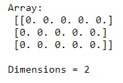
Explanation: np.empty() function will generate the numpy array by setting all elements =0 based on given shape. It works same as np.zeros() function.
Output:

F7). full() function:

a = np.full((2,3,4), 999, dtype=int)
print("Array:\n", a)
print("\nArray Dimensions = ", a.ndim)
print("Array Shape = ", a.shape)

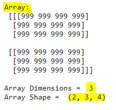
Explanation: np.full() function will be useful when we want to create numpy array with given value and given dimensions. Here 999 is the value we want to set all elements in the array and (2,3,4) is the dimensions we want to create numpy array.
Output:

F8). transpose() function:

print(" ***** Original Array: ***** \n",a)
a = np.array(np.arange(12).reshape(3,4))
print("\nShape of Original Array:",a.shape)
print("Dimensions of Original Array:",a.ndim)


print("\n ***** Transposed Array: ***** \n",b)
#b = a.transpose()  --> #same as below
b = np.transpose(a)
print("\nShape of Transposed Array:",b.shape)
print("Dimensions of Transposed Array:",b.ndim)

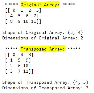
Explanation: By using transpose() function, we can change the rows into columns and columns into rows of a numpy array or matrix. We can imagine like rotating array. This is very useful in mathematical area and Data Science field.
Ex: In below example we have original array with shape= (3,4) i.e. 3 rows, 4 columns. After applying transpose() function now we have array shape = (4,3) i.e. 4 rows, 3 columns. We can use a.transpose(), np.transpose(a)either of the ways to get this required output. First row (0,1,2,3) in the original array becomes first column (0,1,2,3) in the transposed array.
Output:

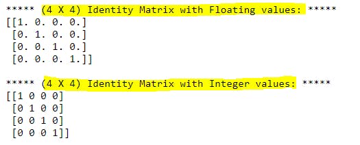
F9). identity() function:

print("***** (4 X 4) Identity Matrix with Floating values: *****")
a = np.identity(4)
print(a)

print("\n***** (4 X 4) Identity Matrix with Integer values: *****")
a = np.identity(4, dtype=int)
print(a)

Explanation: np.identity() function is used to create n X n square identity matrix(2D array) where all diagonal elements set to 1 and rest of the elements set to 0. By default data type of elements will be floating numbers. We can use dtype=int parameter to convert floating numbers into integer values. This matrix will be very useful in mathematics and Data science fields. Here n=4 so 4 X 4 square identity matrix will be created.
Output:

F10). eye() function:

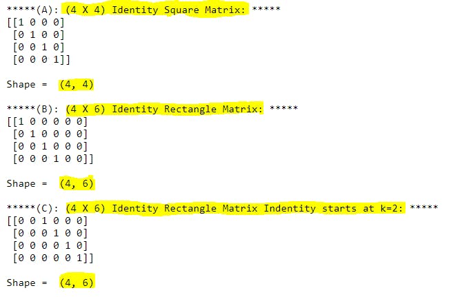
print("*****(A): (4 X 4) Identity Square Matrix: *****")
a = np.eye(4, dtype=int)
print(a)
print("\nShape = ",a.shape)

print("\n*****(B): (4 X 6) Identity Rectangle Matrix: *****")
a = np.eye(4,6, dtype=int)
print(a)
print("\nShape = ",a.shape)

print("\n*****(C): (4 X 6) Identity Rectangle Matrix Indentity starts at k=2: *****")
a = np.eye(4,6,k=2, dtype=int)
print(a)
print("\nShape = ",a.shape)

Explanation: With np.eye() function we can able to create square identity matrix as well as rectangle identity matrix based on shape we provide to the function.
Ex - A We have given np.eye(4, dtype=int) and the output will be 4 X 4 square identity matrix where all diagonal elements will be set to 1 and rest of the elements will be set to 0 and diagonal starts at (0,0) position.
Ex - B We have given np.eye(4,6, dtype=int) and the output will be 4 X 6 rectangle identity matrix where all diagonal elements will be set to 1 and rest of the elements will be set to 0 and diagonal starts at (0,0) position. But last 2 columns will not be having 1 in the diagonal as this array is not square matrix.
Ex - C We have given np.eye(4,6,k=2, dtype=int) and the output will be 4 X 6 rectangle identity matrix where all diagonal elements will be set to 1 and rest of the elements will be set to 0 and diagonal starts at (0,2) position because we set k=2 and identity diagonal will starts from k=2. But first 2 columns will not be having 1 in the diagonal as this array is not square matrix and we mentioned to start from k=2.

Output:

---

G). Copying or Duplicating Numpy arrays:

We have totally 3 ways to copying or duplicating the numpy arrays.

• = : With assignment operator we can assign different variables to same numpy array but multiple copies of arrays will not get create.
• view() : This function also called as shallow copy and it will not create a new copy of numpy array.
• copy() : This function will generate a new copy of numpy array.

Before jumping into the array copying concepts, we need to understand the id() function, base attribute. With the help of these 2 we can easily understand the array copying concepts.

G1). ID function, Base attributes of Numpy Array :

print("*****(A): ID() function: *****")
print("ID(5): ", id(5))
x = 5
print("ID(X): ", id(x))
y = x
print("ID(Y): ", id(y))
z = [1,2,3]
print("ID(Z): ", id(z))

print("\n*****(B): base attribute: *****")
p=np.arange(10)
print("P.Base = ", p.base)
print("P.Base is None = ", p.base is None)

q = p[5:]
print("\nQ.Base = ", q.base)
print("Q.Base is P = ", q.base is p)
print("Q.Base None = ", q.base is None)

r = p
print("\nR.Base = ", r.base)
print("R.Base is P = ", r.base is p)
print("R.Base is None = ", r.base is None)

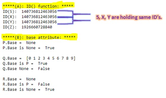
Explanation: Ex - A : id() : This function is used to print the identity of a particular python object(it can be Variable, List, Tuple, Dictionary, .....) and it is a integer value. This value will be remain same for an object lifetime in the given program.
Ex -A-Output : In the above example value 5 is having some ID, 5 is assigned to variable x and x is also holding the same ID. Variable x is assigned to variable y and y also holds the same ID. It means if the one value assigned to multiple variables with = assignment operator then those objects also holds the same ID's. ID for list z is different then x, y ID's.
Ex - B : base: This attribute is used to check the base memory of given object is derived from any other object or not. If the given object is not derived from other objects then the base = None.
Ex -B-Output : In the above example p is a numpy array having values from 0 to 9. This is not based or derived from any of existing object and it is created by numpy function so p.base = None. q is a sub array of p so it is derived from memory of p. Thats why q.base = p i.e. numpy array from 0 to 9. r is assigned to p but not subpart of p so r.base = None same as p.base = None .

Output:

G2). Simple Assignment =:

print("*****(A): Create numpy array and make a copy with assignment operator: *****")
a = np.array(np.arange(10))
b = a
print("Original_Array A:\n",a)
print("\nTemp_Array B:\n",b)

print("\n*****(B): Check the ID, Base of each array before modification: *****")
print("ID of A :",id(a))
print("ID of B :",id(b))
print("\nB is A:",b is a)
print("A is B:",a is b)
print("\nB.base is A:",b.base is a)
print("A.base is B:",a.base is b)

print("\n*****(C): Modify the Temp array and check the ID, Base of each array: *****")
b[0] = 9999
print("Original_Array A:\n",a)
print("\nTemp_Array B:\n",b)
print("\nID of A :",id(a))
print("ID of B :",id(b))

print("\n*****(D): Modify the Original array and check the ID, Base of each array: *****")
a[0] = 2222
print("Original_Array A:\n",a)
print("\nTemp_Array B:\n",b)
print("\nID of A :",id(a))
print("ID of B :",id(b))

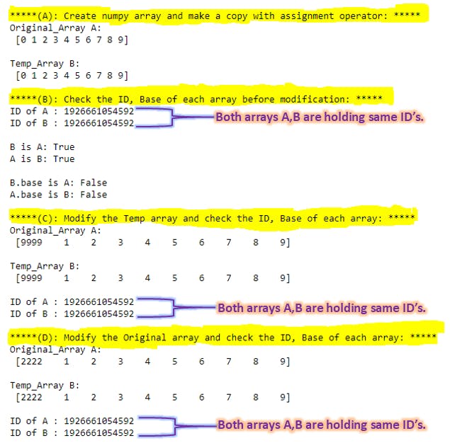
Explanation: Simple assignments make no copy of objects or their data.
In Section-A: we just have created numpy array as a = np.array(np.arange(10)) and simply assigned b = a. Lets consider a is original array and b is temporary array for our understanding.
In Section-B: we are trying to check the memory location of a, b variables using id() function and a, b variables are having same ID. Using is keyword we can check a, b variables are same and no hidden view has been created and b is a , a is b are giving True as output. Using base attribute we can check one variable is derived or sliced from another variable. Here b.base is a, a.base is b are giving False as an output because none of the arrays are derived or sliced from another variable.
In Section-C: we are trying to modify the one index in temporary array b as b[0] = 9999. Now if we see original array also got modified and both a, b arrays ID's are also same. Which means with = assignment no second copy of the array has been created.
In Section-D: we are trying to modify the one index in original array a as a[0] = 2222. Now if we see temporary array also got modified and both a, b arrays ID's are also same. Which means with = assignment no second copy of the array has been created.
Output:

G3). View() or Shallow copy:

print("*****(A): Create numpy array and make a copy with view() function: *****")
a = np.array(np.arange(10))
b = a.view()
print("Original_Array A:\n",a)
print("\nTemp_Array B:\n",b)

print("\n*****(B): Check the ID, Base of each array before modification: *****")
print("ID of A :",id(a))
print("ID of B :",id(b))
print("\nB is A:",b is a)
print("A is B:",a is b)
print("\nB.base is A:",b.base is a)
print("A.base is B:",a.base is b)

print("\n*****(C): Modify the Temp array and check the ID, Base of each array: *****")
b[0] = 9999
print("Original_Array A:\n",a)
print("\nTemp_Array B:\n",b)
print("\nID of A :",id(a))
print("ID of B :",id(b))

print("\n*****(D): Modify the Original array and check the ID, Base of each array: *****")
a[0] = 2222
print("Original_Array A:\n",a)
print("\nTemp_Array B:\n",b)
print("\nID of A :",id(a))
print("ID of B :",id(b))

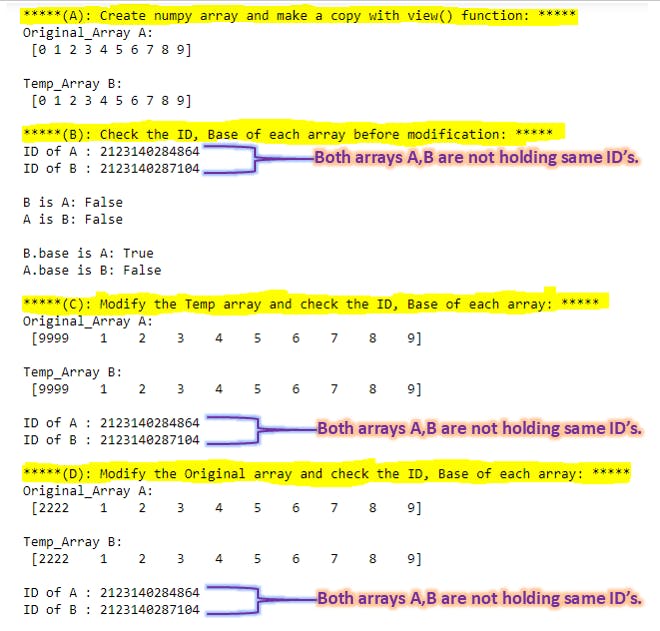
Explanation: view() function will create a shallow copy for a variable. Shallow copy means not a complete copy.
In Section-A: we just have created numpy array as a = np.array(np.arange(10)) and created temp array as b = a.view(). Lets consider a is original array and b is temporary array for our understanding.
In Section-B: we are trying to check the memory location of a, b variables using id() function and a, b variables are not having same ID. Using is keyword we can check a, b variables are not same and hidden view has been created and b is a , a is b are giving False as output because there is a shallow copy has been created due to this ID's are not same. Using base attribute we can check one variable is derived or sliced from another variable. Here b.base is a is True because b is derived from a. a.base is b are giving False as an output because a is not derived or sliced from b.
In Section-C: we are trying to modify the one index in temporary array b as b[0] = 9999. Now if we see original array also got modified but both a, b arrays ID's are not same this is what shallow copy means. Which means with view() function ID's will get differ but modifying one array will reflect the other.
In Section-D: we are trying to modify the one index in original array a as a[0] = 2222. Now if we see temporary array also got modified but both a, b arrays ID's are not same this is what shallow copy means. Which means with view() function ID's will get differ but modifying one array will reflect the other.
Output:

G4). Copy() or Deep copy:

print("*****(A): Create numpy array and make a copy with copy() function: *****")
a = np.array(np.arange(10))
b = a.copy()
print("Original_Array A:\n",a)
print("\nTemp_Array B:\n",b)

print("\n*****(B): Check the ID, Base of each array before modification: *****")
print("ID of A :",id(a))
print("ID of B :",id(b))
print("\nB is A:",b is a)
print("A is B:",a is b)
print("\nB.base is A:",b.base is a)
print("A.base is B:",a.base is b)

print("\n*****(C): Modify the Temp array and check the ID, Base of each array: *****")
b[0] = 9999
print("Original_Array A:\n",a)
print("\nTemp_Array B:\n",b)
print("\nID of A :",id(a))
print("ID of B :",id(b))

print("\n*****(D): Modify the Original array and check the ID, Base of each array: *****")
a[0] = 2222
print("Original_Array A:\n",a)
print("\nTemp_Array B:\n",b)
print("\nID of A :",id(a))
print("ID of B :",id(b))

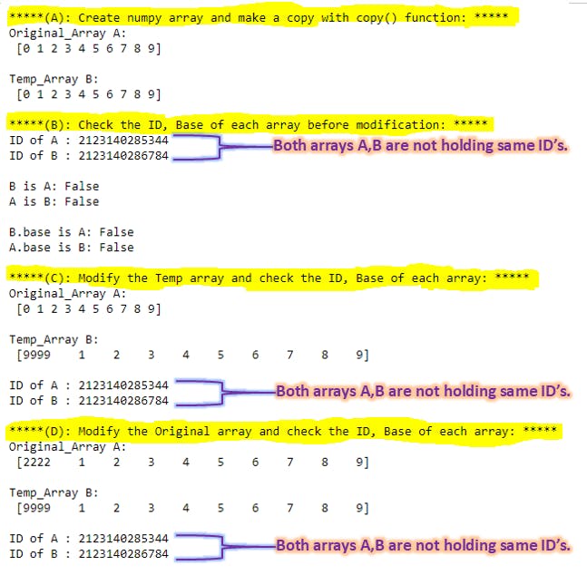
Explanation: copy() function will create a deep copy for a variable. Deep copy means a complete separate copy.
In Section-A: we just have created numpy array as a = np.array(np.arange(10)) and created temp array as b = a.view(). Lets consider a is original array and b is temporary array for our understanding.
In Section-B: we are trying to check the memory location of a, b variables using id() function and a, b variables are not having same ID. Using is keyword we can check a, b variables are not same and separate view has been created and b is a , a is b are giving False as output because there is a deep separate copy has been created due to this ID's are not same. Using base attribute we can check one variable is derived or sliced from another variable. Here b.base is a is False because b is a deep copy of a and not derived from a. a.base is b are giving False as an output because a is not derived or sliced from b.
In Section-C: we are trying to modify the one index in temporary array b as b[0] = 9999. Now if we see original array is not modified. This is because a, b are two deep(separate) copies now and both a, b arrays ID's are not same this is what Deep copy means. Which means with copy() function ID's will get differ and modifying one array will not reflect the other.
In Section-D: we are trying to modify the one index in original array a as a[0] = 2222. Now if we see original array is not modified. This is because a, b are two deep(separate) copies now and both a, b arrays ID's are not same this is what Deep copy means. Which means with copy() function ID's will get differ and modifying one array will not reflect the other.
Output:

---

H). Broadcasting in Numpy

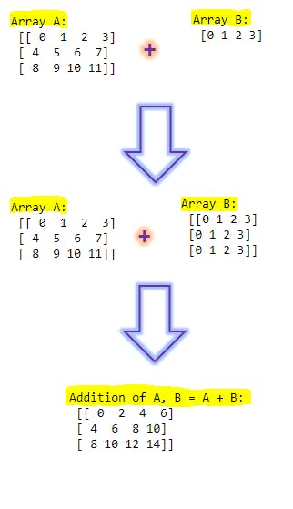
• Braodcasting allows to perform arithmetic operations on arrays of different shapes.
• In 2 different shapes of arrays, we are transforming smaller array shape into larger array shape and then perform given operations. In this process the smaller array will be broadcasted automatically.
• For Broadcasting we wont use any additional keyword, bydefault smaller array will converted into bigger array shape.

H1). Broadcasting Example-1:

a = np.array(np.arange(12).reshape(3,4))
print("\nArray A: \n", a)

b = np.array(np.arange(4))
print("\nArray B: \n", b)

c = a + b
print("\nArray C = A + B :\n",c)

print("\nArray A dimensions: ", a.shape)
print("Array B dimensions: ", b.shape)
print("Array C dimensions: ", c.shape)

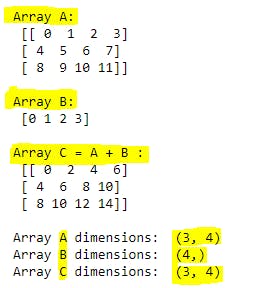
Explanation: With a = np.array(np.arange(12).reshape(3,4)) we have created 3 X 4 dimension array and with b = np.array(np.arange(4)) we have created 1 dimensional array having 4 values in it. Now when we try to print print("\nArray C = A + B :\n",c) we get output array also in 3 X 4 dimension. Here Array B got converted into 3 X 4 dimension automatically without using any extra keyword. But here column size should match else this broadcasting will not work. Here Array A is having 3 rows, 4 columns and Array B is having 1 row, 4 columns so columns size is matching and broadcasting has happened automatically when we apply arithmetic operations on Numpy arrays.
Output:

H2). Step by step explanation for Broadcasting process:

print("\nLet's see how array B has broadcasted into given Bigger array shape:")
c = np.array([b,b,b])
#c = np.array([b]*3)
#c= np.array([b,]*3)
print(c)

Explanation: The above explanation will be same and here if we want to manually make small size array into bigger array without broadcast we can use any of the commands above. c = np.array([b,b,b]) or c = np.array([b]*3) or c= np.array([b,]*3).
Output:

---

I). Numerical operations on Numpy Array:

• In this section we will be working on adding a number to numpy array or multiplying a number with numpy array and adding or multiplying with value or numpy array.
• To multiply 2 numpy arrays, left side array columns count and right side array rows count should match.
• To add 2 numpy arrays, shape of both arrays should match else broadcast will apply for smaller size array.

I1). Numpy array with any numerical value:

a = np.array(np.arange(40,60).reshape(4,5))
print("Original Array :\n",a)

#Symbols: +, -, *, /, **

print("\nArray+10 : Addition of array and value :\n",a+10)
print("\nArray*10 : Multiplication of array and value :\n",a*10)

Explanation: We can use any of the arithmetic operations(+, -, , /, *) mentioned above. If we add( or any arithmetic operation) to numpy array with any given value then the operation will be performed in each element in array with given number and gives the output in same indexing position.

Output: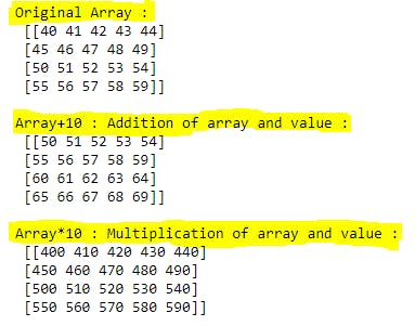

I2). 2 Numpy arrays with same shape: Without Broadcast:

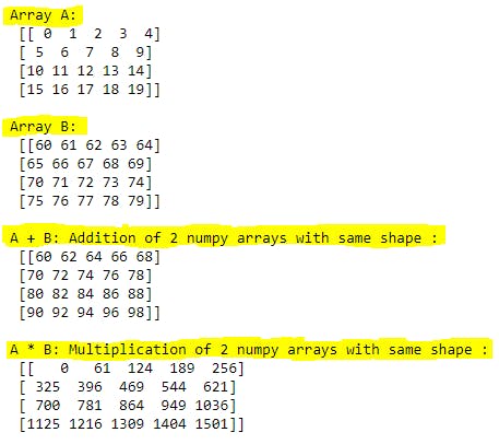
a = np.array(np.arange(20).reshape(4,5))
print("Array A:\n",a)

b = np.array(np.arange(60,80).reshape(4,5))
print("\nArray B:\n",b)

print("\nA + B: Addition of 2 numpy arrays with same shape :\n", a + b)
print("\nA * B: Multiplication of 2 numpy arrays with same shape :\n", a * b)

Explanation: Here 2 numpy arrays are having same size and no broadcast required here. If we add (or arithmetic operation) on 2 arrays, then given operation will be performed on corresponding index elements in each array.
Ex: (0,0) Index element in Array A is 0 and in Array B is 60. If the given operation is + then in the output array will be having 0 + 60 = 60 in the index (0,0). Same will be applicable with all the arithmetic operations. If operation is * then 0 * 60 = 0 in the (0,0) index.
Output:

I3). 2 Numpy arrays with same shape: With Broadcast:

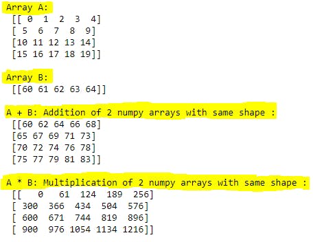
a = np.array(np.arange(20).reshape(4,5))
print("Array A:\n",a)

b = np.array(np.arange(60,65).reshape(1,5))
print("\nArray B:\n",b)

print("\nA + B: Addition of 2 numpy arrays with same shape :\n", a + b)
print("\nA * B: Multiplication of 2 numpy arrays with same shape :\n", a * b)

Explanation: Shape of Array A is (4,5) and Shape of Array B is (1,5). If we apply any arithmetic operation between these 2 arrays then smallest array(Array B) will be broadcasted automatically into shape (4,5) and then operations will be performed. We ahev already covered the broadcasting process in above section.
Note: If and only if smallest array's rows count =1 and columns count should match with largest array's columns count to perform these kind of arithmetic operations.
Output:

---

J). Matrices vs Numpy Ndarray :

• Numpy matrix class is a subset of Numpy ndarray class.
• Numpy arrays can be converted into Matrix by using mat() or matrix() function.
• Matrix objects are strictly 2-Dimensional arrays we cann't create any other dimensional arrays in Matrix objects. But ndarray objects can be any dimensional arrays (1D, 2D, 3D,....., nD).
• We can observe the difference between Matrix vs ndarrays by using * or multiplication operation.

J1). Creation of Matrix, Ndarrays:

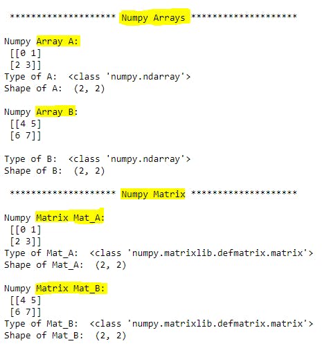
print('\n', "*" * 20,'Numpy Arrays', "*" * 20, '\n')

a = np.array(np.arange(4).reshape(2,2))
print("Numpy Array A:\n",a)
print("Type of A: ",type(a))
print("Shape of A: ",np.shape(a))

b = np.array(np.arange(4,8).reshape(2,2))
print("\nNumpy Array B:\n",b)
print("\nType of B: ",type(b))
print("Shape of B: ",np.shape(b))

print('\n', "*" * 20,'Numpy Matrix', "*" * 20, '\n')

Mat_A = np.matrix(a)
print("Numpy Matrix Mat_A:\n",Mat_A)
print("Type of Mat_A: ",type(Mat_A))
print("Shape of Mat_A: ",np.shape(Mat_A))

Mat_B = np.matrix(b)
print("\nNumpy Matrix Mat_B:\n",Mat_B)
print("Type of Mat_B: ",type(Mat_B))
print("Shape of Mat_B: ",np.shape(Mat_B))

Explanation: We have created Numpy arrays as usual. By using mat() or matrix() functions we can convert the Numpy array into Numpy Matrix. We can cross check the classes using type() method.
Output:

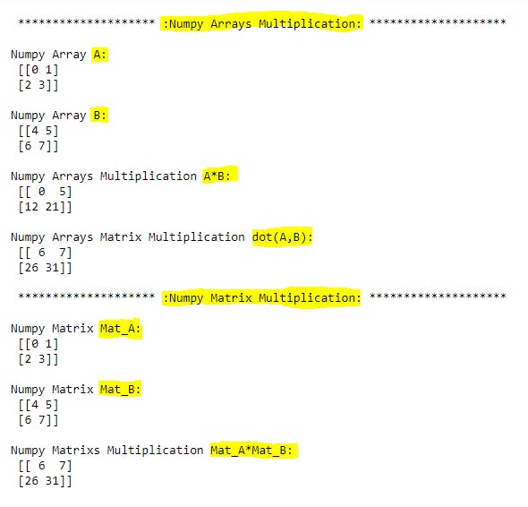
J2). Numpy Arrays, Matrix multiplication:

print('\n', "*" * 20,':Numpy Arrays Multiplication:', "*" * 20, '\n')

a = np.array(np.arange(4).reshape(2,2))
b = np.array(np.arange(4,8).reshape(2,2))
print("Numpy Array A:\n",a)
print("\nNumpy Array B:\n",b)
print("\nNumpy Arrays Multiplication A*B:\n",a*b)
print("\nNumpy Arrays Matrix Multiplication dot(A,B):\n",np.dot(a,b))

print('\n', "*" * 20,':Numpy Matrix Multiplication:', "*" * 20, '\n')

Mat_A = np.matrix(a)
Mat_B = np.matrix(b)
print("Numpy Matrix Mat_A:\n",Mat_A)
print("\nNumpy Matrix Mat_B:\n",Mat_B)
print("\nNumpy Matrixs Multiplication Mat_A*Mat_B:\n",Mat_A*Mat_B)

Explanation: We can clearly observe that with * (multiplication) operation there is difference between arrays and matrices. In arrays * operation takes places on respective index of arrays. Index of (0,0) in Array A is 0 and Array B is4 then in output it will be 0 X 4 = 0. In Matrix multiplication we can see the output value at index (0,0) = (A[0,0] X B[0,0]) + (A[0,1] x B[1,0]) = 6. More details on matrix multiplications in wikipedia page here. Same operation can be done on Numpy Arrays by using dot() method.
Output:

---

K). Numpy inbuilt functions :

• Numpy Statistical functions: min(), max(), mean(), mode(), std(), var(), ..
• Numpy Trigonometric, Exponential, Logarithmic functions: sin(), cos(), tan(), exp(), log(), ..
• Numpy Rounding functions: round(), ceil(), floor()

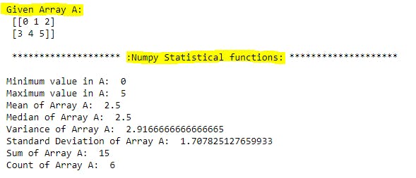
K1). Numpy Statistical functions:

a = np.array(np.arange(6).reshape(2,3))
print("Given Array A:\n",a)

print('\n', "*" * 20,':Numpy Statistical functions:', "*" * 20)
print("\nMinimum value in A: ", np.min(a))
print("Maximum value in A: ", np.max(a))
print("Mean of Array A: ", np.mean(a))
print("Median of Array A: ", np.median(a))
print("Variance of Array A: ", np.var(a))
print("Standard Deviation of Array A: ", np.std(a))
print("Sum of Array A: ", np.sum(a))
print("Count of Array A: ", np.size(a))

Explanation: In this statistical functions are very useful in data analysis and data science domains to figure out the data distribution in given column to take business decisions.
Output:

K2). Numpy Trigonometric, Exponential, Logarithmic functions:

a = np.array(np.arange(6).reshape(2,3))
print("Given Array A:\n",a)

print('\n', "*" * 20,':Numpy Trigonometric functions:', "*" * 20)
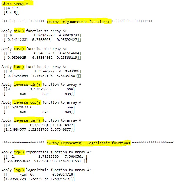
print("\nApply sin() function to array A: \n", np.sin(a))
print("\nApply cos() function to array A: \n", np.cos(a))
print("\nApply tan() function to array A: \n", np.tan(a))
print("\nApply inverse sin() function to array A: \n", np.arcsin(a))
print("\nApply inverse cos() function to array A: \n", np.arccos(a))
print("\nApply inverse tan() function to array A: \n", np.arctan(a))

print('\n\n', "*" * 20,':Numpy Exponential, Logarithmic functions:', "*" * 20)
print("\nApply exp() exponential function to array A: \n", np.exp(a))
print("\nApply log() logarithmic function to array A: \n", np.log(a))

Explanation: Trigonometric, Exponential and Logarithmic functions are very useful in Data Science and Machine learning fields.
Output:

K3). Numpy Rounding functions:

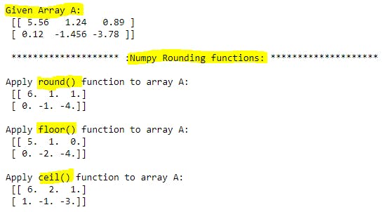
a = np.array([5.56, 1.24, 0.89, 0.12, -1.456, -3.78]).reshape(2,3)
print("Given Array A:\n",a)

print('\n', "*" * 20,':Numpy Rounding functions:', "*" * 20)
print("\nApply round() function to array A: \n", np.round(a))
print("\nApply floor() function to array A: \n", np.floor(a))
print("\nApply ceil() function to array A: \n", np.ceil(a))

Explanation: These rounding functions are very useful in scientific calculations and Machine learning concepts.
round() function will make the element or number to nearest rounding number(it will increase or decrease the number to make it rounded to nearest number).
floor() function will round the given number to nearest small number. (for 5.56 the nearest small number will be 5.0).
ceil function will round the given number to nearest big number. (for 0.12 the nearest big number will be 1.0).
Output:

---

Conclusion:

I hope you have learned Numpy concepts with simple examples.
Happy Learning...!!